Introduction
This manual explains how to use Draw, the test harness for Open CASCADE Technology (OCCT). Draw is a command interpreter based on TCL and a graphical system used to test and demonstrate Open CASCADE Technology modeling libraries.
Overview
Draw is a test harness for Open CASCADE Technology. It provides a flexible and easy to use means of testing and demonstrating the OCCT modeling libraries.
Draw can be used interactively to create, display and modify objects such as curves, surfaces and topological shapes.
Scripts may be written to customize Draw and perform tests. New types of objects and new commands may be added using the C++ programming language.
Draw consists of:
- A command interpreter based on the TCL command language.
- A 3d graphic viewer based on the X system.
- A basic set of commands covering scripts, variables and graphics.
- A set of geometric commands allowing the user to create and modify curves and surfaces and to use OCCT geometry algorithms. This set of commands is optional.
- A set of topological commands allowing the user to create and modify BRep shapes and to use the OCCT topology algorithms.
There is also a set of commands for each delivery unit in the modeling libraries:
- GEOMETRY,
- TOPOLOGY,
- ADVALGOS,
- GRAPHIC,
- PRESENTATION.
Contents of this documentation
This documentation describes:
- The command language.
- The basic set of commands.
- The graphical commands.
- The Geometry set of commands.
- The Topology set of commands.
- OCAF commands.
- Data Exchange commands
- Shape Healing commands
This document is a reference manual. It contains a full description of each command. All descriptions have the format illustrated below for the exit command.
Terminates the Draw, TCL session. If the commands are read from a file using the source command, this will terminate the file.
Example:
# this is a very short example
exit
Getting started
Install Draw and launch Emacs. Get a command line in Emacs using Esc x and key in woksh.
All DRAW Test Harness can be activated in the common executable called DRAWEXE. They are grouped in toolkits and can be loaded at run-time thereby implementing dynamically loaded plug-ins. Thus, it is possible to work only with the required commands adding them dynamically without leaving the Test Harness session.
Declaration of available plug-ins is done through the special resource file(s). The pload command loads the plug-in in accordance with the specified resource file and activates the commands implemented in the plug-in.
Launching DRAW Test Harness
Test Harness executable DRAWEXE is located in the $CASROOT/<platform>/bin directory (where <platform> is Win for Windows and Linux for Linux operating systems). Prior to launching it is important to make sure that the environment is correctly setup (usually this is done automatically after the installation process on Windows or after launching specific scripts on Linux).
Plug-in resource file
Open CASCADE Technology is shipped with the DrawPlugin resource file located in the $CASROOT/src/DrawResources directory.
The format of the file is compliant with standard Open CASCADE Technology resource files (see the Resource_Manager.hxx file for details).
Each key defines a sequence of either further (nested) keys or a name of the dynamic library. Keys can be nested down to an arbitrary level. However, cyclic dependencies between the keys are not checked.
Example: (excerpt from DrawPlugin):
OCAF : VISUALIZATION, OCAFKERNEL
VISUALIZATION : AISV
OCAFKERNEL : DCAF
DCAF : TKDCAF
AISV : TKViewerTest
Activation of commands implemented in the plug-in
To load a plug-in declared in the resource file and to activate the commands the following command must be used in Test Harness:
pload [-PluginFileName] [[Key1] [Key2]...]
Where:
- -PluginFileName – defines the name of a plug-in resource file (prefix "-" is mandatory) described above. If this parameter is omitted then the default name DrawPlugin is used.
- Key – defines the key(s) enumerating plug-ins to be loaded. If no keys are specified then the key named DEFAULT is used (if there is no such key in the file then no plug-ins are loaded).
According to the OCCT resource file management rules, to access the resource file the environment variable CSF_PluginFileNameDefaults (and optionally CSF_PluginFileNameUserDefaults) must be set and point to the directory storing the resource file. If it is omitted then the plug-in resource file will be searched in the $CASROOT/src/DrawResources directory.
Draw[] pload -DrawPlugin OCAF
This command will search the resource file DrawPlugin using variable CSF_DrawPluginDefaults (and CSF_DrawPluginUserDefaults) and will start with the OCAF key. Since the DrawPlugin is the file shipped with Open CASCADE Technology it will be found in the $CASROOT/src/DrawResources directory (unless this location is redefined by user's variables). The OCAF key will be recursively extracted into two toolkits/plug-ins: TKDCAF and TKViewerTest (e.g. on Windows they correspond to TKDCAF.dll and TKViewerTest.dll). Thus, commands implemented for Visualization and OCAF will be loaded and activated in Test Harness.
Draw[] pload (equivalent to pload -DrawPlugin DEFAULT).
This command will find the default DrawPlugin file and the DEFAULT key. The latter finally maps to the TKTopTest toolkit which implements basic modeling commands.
The Command Language
Overview
The command language used in Draw is Tcl. Tcl documentation such as "TCL and the TK Toolkit" by John K. Ousterhout (Addison-Wesley) will prove useful if you intend to use Draw extensively.
This chapter is designed to give you a short outline of both the TCL language and some extensions included in Draw. The following topics are covered:
- Syntax of the TCL language.
- Accessing variables in TCL and Draw.
- Control structures.
- Procedures.
Syntax of TCL
TCL is an interpreted command language, not a structured language like C, Pascal, LISP or Basic. It uses a shell similar to that of csh. TCL is, however, easier to use than csh because control structures and procedures are easier to define. As well, because TCL does not assign a process to each command, it is faster than csh.
The basic program for TCL is a script. A script consists of one or more commands. Commands are separated by new lines or semicolons.
set a 24
set b 15
set a 25; set b 15
Each command consists of one or more words; the first word is the name of a command and additional words are arguments to that command.
Words are separated by spaces or tabs. In the preceding example each of the four commands has three words. A command may contain any number of words and each word is a string of arbitrary length.
The evaluation of a command by TCL is done in two steps. In the first step, the command is parsed and broken into words. Some substitutions are also performed. In the second step, the command procedure corresponding to the first word is called and the other words are interpreted as arguments. In the first step, there is only string manipulation, The words only acquire meaning in the second step by the command procedure.
The following substitutions are performed by TCL:
Variable substitution is triggered by the $ character (as with csh), the content of the variable is substituted; { } may be used as in csh to enclose the name of the variable.
Example:
# set a variable value
set file documentation
puts $file #to display file contents on the screen
# a simple substitution, set psfile to documentation.ps
set psfile $file.ps
puts $psfile
# another substitution, set pfile to documentationPS
set pfile ${file}PS
# a last one,
# delete files NEWdocumentation and OLDdocumentation
foreach prefix {NEW OLD} {rm $prefix$file}
Command substitution is triggered by the [ ] characters. The brackets must enclose a valid script. The script is evaluated and the result is substituted.
Compare command construction in csh.
Example:
set degree 30
set pi 3.14159265
# expr is a command evaluating a numeric expression
set radian [expr $pi*$degree/180]
Backslash substitution is triggered by the backslash character. It is used to insert special characters like $, [ , ] , etc. It is also useful to insert a new line, a backslash terminated line is continued on the following line.
TCL uses two forms of quoting to prevent substitution and word breaking.
Double quote quoting enables the definition of a string with space and tabs as a single word. Substitutions are still performed inside the inverted commas " ".
Example:
# set msg to ;the price is 12.00;
set price 12.00
set msg ;the price is $price;
Braces quoting prevents all substitutions. Braces are also nested. The main use of braces is to defer evaluation when defining procedures and control structures. Braces are used for a clearer presentation of TCL scripts on several lines.
Example:
set x 0
# this will loop for ever
# because while argument is ;0 < 3;
while ;$x < 3; {set x [expr $x+1]}
# this will terminate as expected because
# while argument is {$x < 3}
while {$x < 3} {set x [expr $x+1]}
# this can be written also
while {$x < 3} {
set x [expr $x+1]
}
# the following cannot be written
# because while requires two arguments
while {$x < 3}
{
set x [expr $x+1]
}
Comments start with a # character as the first non-blank character in a command. To add a comment at the end of the line, the comment must be preceded by a semi-colon to end the preceding command.
Example:
# This is a comment
set a 1 # this is not a comment
set b 1; # this is a comment
The number of words is never changed by substitution when parsing in TCL. For example, the result of a substitution is always a single word. This is different from csh but convenient as the behavior of the parser is more predictable. It may sometimes be necessary to force a second round of parsing. eval accomplishes this: it accepts several arguments, concatenates them and executes the resulting script.
Example:
# I want to delete two files
set files ;foo bar;
# this will fail because rm will receive only one argument
# and complain that ;foo bar; does not exit
exec rm $files
# a second evaluation will do it
Accessing variables in TCL and Draw
TCL variables have only string values. Note that even numeric values are stored as string literals, and computations using the expr command start by parsing the strings. Draw, however, requires variables with other kinds of values such as curves, surfaces or topological shapes.
TCL provides a mechanism to link user data to variables. Using this functionality, Draw defines its variables as TCL variables with associated data.
The string value of a Draw variable is meaningless. It is usually set to the name of the variable itself. Consequently, preceding a Draw variable with a $ does not change the result of a command. The content of a Draw variable is accessed using appropriate commands.
There are many kinds of Draw variables, and new ones may be added with C++. Geometric and topological variables are described below.
Draw numeric variables can be used within an expression anywhere a Draw command requires a numeric value. The expr command is useless in this case as the variables are stored not as strings but as floating point values.
Example:
# dset is used for numeric variables
# pi is a predefined Draw variable
dset angle pi/3 radius 10
point p radius*cos(angle) radius*sin(angle) 0
It is recommended that you use TCL variables only for strings and Draw for numerals. That way, you will avoid the expr command. As a rule, Geometry and Topology require numbers but no strings.
set, unset
Syntax:
set varname [value]
unset varname [varname varname ...]
set assigns a string value to a variable. If the variable does not already exist, it is created.
Without a value, set returns the content of the variable.
unset deletes variables. It is also used to delete Draw variables.
Example:
set a "Hello world"
set b "Goodbye"
set a
== "Hello world"
unset a b
set a
Note, that the set command can set only one variable, unlike the dset command.
dset, dval
Syntax
dset var1 value1 vr2 value2 ...
dval name
dset assigns values to Draw numeric variables. The argument can be any numeric expression including Draw numeric variables. Since all Draw commands expect a numeric expression, there is no need to use $ or expr. The dset command can assign several variables. If there is an odd number of arguments, the last variable will be assigned a value of 0. If the variable does not exist, it will be created.
dval evaluates an expression containing Draw numeric variables and returns the result as a string, even in the case of a single variable. This is not used in Draw commands as these usually interpret the expression. It is used for basic TCL commands expecting strings.
Example:
# z is set to 0
dset x 10 y 15 z
== 0
# no $ required for Draw commands
point p x y z
# "puts" prints a string
puts ;x = [dval x], cos(x/pi) = [dval cos(x/pi)];
== x = 10, cos(x/pi) = -0.99913874099467914
Note, that in TCL, parentheses are not considered to be special characters. Do not forget to quote an expression if it contains spaces in order to avoid parsing different words. (a + b) is parsed as three words: "(a + b)" or (a+b) are correct.
del, dall
Syntax:
del varname_pattern [varname_pattern ...]
dall
del command does the same thing as unset, but it deletes the variables matched by the pattern.
dall command deletes all variables in the session.
lists
TCL uses lists. A list is a string containing elements separated by spaces or tabs. If the string contains braces, the braced part accounts as one element.
This allows you to insert lists within lists.
Example:
# a list of 3 strings
;a b c;
# a list of two strings the first is a list of 2
;{a b} c;
Many TCL commands return lists and foreach is a useful way to create loops on list elements.
Control Structures
TCL allows looping using control structures. The control structures are implemented by commands and their syntax is very similar to that of their C counterparts (if, while, switch, etc.). In this case, there are two main differences between TCL and C:
- You use braces instead of parentheses to enclose conditions.
- You do not start the script on the next line of your command.
if
Syntax
if condition script [elseif script .... else script]
If evaluates the condition and the script to see whether the condition is true.
Example:
if {$x > 0} {
puts ;positive;
} elseif {$x == 0} {
puts ;null;
} else {
puts ;negative;
}
while, for, foreach
Syntax:
while condition script
for init condition reinit script
foreach varname list script
The three loop structures are similar to their C or csh equivalent. It is important to use braces to delay evaluation. foreach will assign the elements of the list to the variable before evaluating the script. \
Example:
# while example
dset x 1.1
while {[dval x] < 100} {
circle c 0 0 x
dset x x*x
}
# for example
# incr var d, increments a variable of d (default 1)
for {set i 0} {$i < 10} {incr i} {
dset angle $i*pi/10
point p$i cos(angle0 sin(angle) 0
}
# foreach example
foreach object {crapo tomson lucas} {display $object}
break, continue
Syntax:
Within loops, the break and continue commands have the same effect as in C.
break interrupts the innermost loop and continue jumps to the next iteration.
Example:
# search the index for which t$i has value ;secret;
for {set i 1} {$i <= 100} {incr i} {
if {[set t$i] == ;secret;} break;
}
Procedures
TCL can be extended by defining procedures using the proc command, which sets up a context of local variables, binds arguments and executes a TCL script.
The only problematic aspect of procedures is that variables are strictly local, and as they are implicitly created when used, it may be difficult to detect errors.
There are two means of accessing a variable outside the scope of the current procedures: global declares a global variable (a variable outside all procedures); upvar accesses a variable in the scope of the caller. Since arguments in TCL are always string values, the only way to pass Draw variables is by reference, i.e. passing the name of the variable and using the upvar command as in the following examples.
As TCL is not a strongly typed language it is very difficult to detect programming errors and debugging can be tedious. TCL procedures are, of course, not designed for large scale software development but for testing and simple command or interactive writing.
proc
Syntax:
proc defines a procedure. An argument may have a default value. It is then a list of the form {argument value}. The script is the body of the procedure.
return gives a return value to the procedure.
Example:
# simple procedure
proc hello {} {
puts ;hello world;
}
# procedure with arguments and default values
proc distance {x1 y1 {x2 0} {y2 0}} {
set d [expr (x2-x1)*(x2-x1) + (y2-y1)*(y2-y1)]
return [expr sqrt(d)]
}
proc fact n {
if {$n == 0} {return 1} else {
return [expr n*[fact [expr n -1]]]
}
}
global, upvar
Syntax:
global varname [varname ...]
upvar varname localname [varname localname ...]
global accesses high level variables. Unlike C, global variables are not visible in procedures.
upvar gives a local name to a variable in the caller scope. This is useful when an argument is the name of a variable instead of a value. This is a call by reference and is the only way to use Draw variables as arguments.
Note that in the following examples the $ character is always necessarily used to access the arguments.
Example:
# convert degree to radian
# pi is a global variable
proc deg2rad (degree} {
return [dval pi*$degree/2.]
}
# create line with a point and an angle
proc linang {linename x y angle} {
upvar linename l
line l $x $y cos($angle) sin($angle)
}
Basic Commands
This chapter describes all the commands defined in the basic Draw package. Some are TCL commands, but most of them have been formulated in Draw. These commands are found in all Draw applications. The commands are grouped into four sections:
- General commands, which are used for Draw and TCL management.
- Variable commands, which are used to manage Draw variables such as storing and dumping.
- Graphic commands, which are used to manage the graphic system, and so pertain to views.
- Variable display commands, which are used to manage the display of objects within given views.
Note that Draw also features a GUI task bar providing an alternative way to give certain general, graphic and display commands
General commands
This section describes several useful commands:
- help to get information,
- source to eval a script from a file,
- spy to capture the commands in a file,
- cpulimit to limit the process cpu time,
- wait to waste some time,
- chrono to time commands.
help
Syntax:
help [command [helpstring group]]
Provides help or modifies the help information.
help without arguments lists all groups and the commands in each group.
Specifying the command returns its syntax and in some cases, information on the command, The joker * is automatically added at the end so that all completing commands are returned as well.
Example:
# Gives help on all commands starting with *a*
source
Syntax:
Executes a file.
The exit command will terminate the file.
spy
Syntax:
Saves interactive commands in the file. If spying has already been performed, the current file is closed. spy without an argument closes the current file and stops spying. If a file already exists, the file is overwritten. Commands are not appended.
If a command returns an error it is saved with a comment mark.
The file created by spy can be executed with the source command.
Example:
# all commands will be saved in the file ;session;
spy session
# the file ;session; is closed and commands are not saved
spy
cpulimit
Syntax:
cpulimit**limits a process after the number of seconds specified in nbseconds. It is used in tests to avoid infinite loops. **cpulimit without arguments removes all existing limits.
Example:
#limit cpu to one hour
cpulimit 3600
wait
Syntax:
Suspends execution for the number of seconds specified in nbseconds. The default value is ten (10) seconds. This is a useful command for a slide show.
# You have ten seconds ...
wait
chrono
Syntax:
chrono [ name start/stop/reset/show/restart/[counter text]]
Without arguments, chrono activates Draw chronometers. The elapsed time ,cpu system and cpu user times for each command will be printed.
With arguments, chrono is used to manage activated chronometers. You can perform the following actions with a chronometer.
- run the chronometer (start).
- stop the chronometer (stop).
- reset the chronometer to 0 (reset).
- restart the chronometer (restart).
- display the current time (show).
- display the current time with specified text (output example - COUNTER text: N), command testdiff will compare such outputs between two test runs (counter).
Example:
chrono
==Chronometers activated.
ptorus t 20 5
==Elapsed time: 0 Hours 0 Minutes 0.0318 Seconds
==CPU user time: 0.01 seconds
==CPU system time: 0 seconds
Variable management commands
isdraw, directory
Syntax:
isdraw varname
directory [pattern]
isdraw tests to see if a variable is a Draw variable. isdraw will return 1 if there is a Draw value attached to the variable.
Use directory to return a list of all Draw global variables matching a pattern.
Example:
set a 1
isdraw a
=== 0
dset a 1
isdraw a
=== 1
circle c 0 0 1 0 5
isdraw c
=== 1
# to destroy all Draw objects with name containing curve
foreach var [directory *curve*] {unset $var}
whatis, dump
Syntax:
whatis varname [varname ...]
dump varname [varname ...]
whatis returns short information about a Draw variable. This is usually the type name.
dump returns a brief type description, the coordinates, and if need be, the parameters of a Draw variable.
Example:
circle c 0 0 1 0 5
whatis c
c is a 2d curve
dump c
***** Dump of c *****
Circle
Center :0, 0
XAxis :1, 0
YAxis :-0, 1
Radius :5
Note The behavior of whatis on other variables (not Draw) is not excellent.
renamevar, copy
Syntax:
renamevar varname tovarname [varname tovarname ...]
copy varname tovarname [varname tovarname ...]
- renamevar changes the name of a Draw variable. The original variable will no longer exist. Note that the content is not modified. Only the name is changed.
- copy creates a new variable with a copy of the content of an existing variable. The exact behavior of copy is type dependent; in the case of certain topological variables, the content may still be shared.
Example:
circle c1 0 0 1 0 5
renamevar c1 c2
# curves are copied, c2 will not be modified
copy c2 c3
datadir, save, restore
Syntax:
datadir [directory]
save variable [filename]
restore filename [variablename]
- datadir without arguments prints the path of the current data directory.
- datadir with an argument sets the data directory path. \
If the path starts with a dot (.) only the last directory name will be changed in the path.
- save writes a file in the data directory with the content of a variable. By default the name of the file is the name of the variable. To give a different name use a second argument.
- restore reads the content of a file in the data directory in a local variable. By default, the name of the variable is the name of the file. To give a different name, use a second argument.
The exact content of the file is type-dependent. They are usually ASCII files and so, architecture independent.
Example:
# note how TCL accesses shell environment variables
# using $env()
datadir
==.
datadir $env(WBCONTAINER)/data/default
==/adv_20/BAG/data/default
box b 10 20 30
save b theBox
==/adv_20/BAG/data/default/theBox
# when TCL does not find a command it tries a shell command
ls [datadir]
== theBox
restore theBox
== theBox
User defined commands
DrawTrSurf provides commands to create and display a Draw geometric variable from a Geom_Geometry object and also get a Geom_Geometry object from a Draw geometric variable name.
DBRep provides commands to create and display a Draw topological variable from a TopoDS_Shape object and also get a TopoDS_Shape object from a Draw topological variable name.
set
In DrawTrSurf package:
void Set(Standard_CString& Name,const gp_Pnt& G) ;
void Set(Standard_CString& Name,const gp_Pnt2d& G) ;
void Set(Standard_CString& Name,
const Handle(Geom_Geometry)& G) ;
void Set(Standard_CString& Name,
const Handle(Geom2d_Curve)& C) ;
void Set(Standard_CString& Name,
const Handle(Poly_Triangulation)& T) ;
void Set(Standard_CString& Name,
const Handle(Poly_Polygon3D)& P) ;
void Set(Standard_CString& Name,
const Handle(Poly_Polygon2D)& P) ;
In DBRep package:
void Set(const Standard_CString Name,
const TopoDS_Shape& S) ;
Example of DrawTrSurf
Handle(Geom2d_Circle) C1 = new Geom2d_Circle
(gce_MakeCirc2d (gp_Pnt2d(50,0,) 25));
DrawTrSurf::Set(char*, C1);
Example of DBRep
TopoDS_Solid B;
B = BRepPrimAPI_MakeBox (10,10,10);
DBRep::Set(char*,B);
get
In DrawTrSurf package:
Handle_Geom_Geometry Get(Standard_CString& Name) ;
In DBRep package:
TopoDS_Shape Get(Standard_CString& Name,
const TopAbs_ShapeEnum Typ = TopAbs_SHAPE,
const Standard_Boolean Complain
= Standard_True) ;
Example of DrawTrSurf
Standard_Integer MyCommand
(Draw_Interpretor& theCommands,
Standard_Integer argc, char** argv)
{......
Handle (Geom_Geometry) aGeom= DrawTrSurf::Get(argv[1]);
}
Example of DBRep
Standard_Integer MyCommand
(Draw_Interpretor& theCommands,
Standard_Integer argc, char** argv)
{......
TopoDS_Solid B = DBRep::Get(argv[1]);
}
Graphic Commands
Graphic commands are used to manage the Draw graphic system. Draw provides a 2d and a 3d viewer with up to 30 views. Views are numbered and the index of the view is displayed in the window’s title. Objects are displayed in all 2d views or in all 3d views, depending on their type. 2d objects can only be viewed in 2d views while 3d objects – only in 3d views correspondingly.
Axonometric viewer
view, delete
Syntax:
view index type [X Y W H]
delete [index]
view is the basic view creation command: it creates a new view with the given index. If a view with this index already exits, it is deleted. The view is created with default parameters and X Y W H are the position and dimensions of the window on the screen. Default values are 0, 0, 500, 500.
As a rule it is far simpler either to use the procedures axo, top, left or to click on the desired view type in the menu under Views in the task bar..
delete deletes a view. If no index is given, all the views are deleted.
Type selects from the following range:
- AXON : Axonometric view
- PERS : Perspective view
- +X+Y : View on both axes (i.e. a top view), other codes are -X+Y, +Y-Z, etc.
- -2D- : 2d view
The index, the type, the current zoom are displayed in the window title .
Example:
# this is the content of the mu4 procedure
proc mu4 {} {
delete
view 1 +X+Z 320 20 400 400
view 2 +X+Y 320 450 400 400
view 3 +Y+Z 728 20 400 400
view 4 AXON 728 450 400 400
}
See also: axo, pers, top, bottom, left, right, front, back, mu4, v2d, av2d, smallview
axo, pers, top, ...
Syntax:
axo
pers
...
smallview type
All these commands are procedures used to define standard screen layout. They delete all existing views and create new ones. The layout usually complies with the European convention, i.e. a top view is under a front view.
- axo creates a large window axonometric view;
- pers creates a large window perspective view;
- top, bottom, left, right, front, back create a large window axis view;
- mu4 creates four small window views: front, left, top and axo.
- v2d creates a large window 2d view.
- av2d creates two small window views, one 2d and one axo
- smallview creates a view at the bottom right of the screen of the given type.
See also: view, delete
mu, md, 2dmu, 2dmd, zoom, 2dzoom
Syntax:
mu [index] value
2dmu [index] value
zoom [index] value
wzoom
- mu (magnify up) increases the zoom in one or several views by a factor of 10%.
- md (magnify down) decreases the zoom by the inverse factor. 2dmu and 2dmd perform the same on one or all 2d views.
- zoom and 2dzoom set the zoom factor to a value specified by you. The current zoom factor is always displayed in the window’s title bar. Zoom 20 represents a full screen view in a large window; zoom 10, a full screen view in a small one.
- wzoom (window zoom) allows you to select the area you want to zoom in on with the mouse. You will be prompted to give two of the corners of the area that you want to magnify and the rectangle so defined will occupy the window of the view.
Example:
# set a zoom of 2.5
zoom 2.5
# magnify by 10%
mu 1
# magnify by 20%
See also: fit, 2dfit
pu, pd, pl, pr, 2dpu, 2dpd, 2dpl, 2dpr
Syntax:
The p_ commands are used to pan. pu and pd pan up and down respectively; pl and pr pan to the left and to the right respectively. Each time the view is displaced by 40 pixels. When no index is given, all views will pan in the direction specified.
# you have selected one anonometric view
pu
# or
pu 1
# you have selected an mu4 view; the object in the third view will pan up
pu 3
See also: fit, 2dfit
fit, 2dfit
Syntax:
fit [index]
2dfit [index]
fit computes the best zoom and pans on the content of the view. The content of the view will be centered and fit the whole window.
When fitting all views a unique zoom is computed for all the views. All views are on the same scale.
Example:
# fit only view 1
fit 1
# fit all 2d views
2dfit
See also: zoom, mu, pu
u, d, l, r
Syntax:
u [index]
d [index]
l [index]
r [index]
u, d, l, r Rotate the object in view around its axis by five degrees up, down, left or right respectively. This command is restricted to axonometric and perspective views.
Example:
focal, fu, fd
Syntax:
focal [f]
fu [index]
fd [index]
- focal changes the vantage point in perspective views. A low f value increases the perspective effect; a high one give a perspective similar to that of an axonometric view. The default value is 500.
- fu and fd increase or decrease the focal value by 10%. fd makes the eye closer to the object.
Example:
Note: Do not use a negative or null focal value.
See also: pers
color
Syntax:
color sets the color to a value. The index of the color is a value between 0 and 15. The name is an X window color name. The list of these can be found in the file rgb.txt in the X library directory.
The default values are: 0 White, 1 Red, 2 Green, 3 Blue, 4 Cyan, 5 Gold, 6 Magenta, 7 Marron, 8 Orange, 9 Pink, 10 Salmon, 11 Violet, 12 Yellow, 13 Khaki, 14 Coral.
Example:
# change the value of blue
color 3 "navy blue"
Note that the color change will be visible on the next redraw of the views, for example, after fit or mu, etc.
dtext
Syntax:
dtext displays a string in all 3d or 2d views. If no coordinates are given, a graphic selection is required. If two coordinates are given, the text is created in a 2d view at the position specified. With 3 coordinates, the text is created in a 3d view.
The coordinates are real space coordinates.
Example:
# mark the origins
dtext 0 0 bebop
dtext 0 0 0 bebop
hardcopy, hcolor, xwd
Syntax:
hardcopy [index]
hcolor index width gray
xwd [index] filename
- hardcopy creates a postcript file called a4.ps in the current directory. This file contains the postscript description of the view index, and will allow you to print the view.
- hcolor lets you change the aspect of lines in the postscript file. It allows to specify a width and a gray level for one of the 16 colors. width is measured in points with default value as 1, gray is the gray level from 0 = black to 1 = white with default value as 0. All colors are bound to the default values at the beginning.
- xwd creates an X window xwd file from an active view. By default, the index is set to1. To visualize an xwd file, use the unix command xwud.
Example:
# all blue lines (color 3)
# will be half-width and gray
hcolor 3 0.5
# make a postscript file and print it
hardcopy
lpr a4.ps
# make an xwd file and display it
xwd theview
xwud -in theview
Note: When more than one view is present, specify the index of the view.
Only use a postscript printer to print postscript files.
See also: color
wclick, pick
Syntax:
wclick
pick index X Y Z b [nowait]
wclick defers an event until the mouse button is clicked. The message just click is displayed.
Use the pick command to get graphic input. The arguments must be names for variables where the results are stored.
- index: index of the view where the input was made.
- X,Y,Z: 3d coordinates in real world.
- b: b is the mouse button 1,2 or 3.
When there is an extra argument, its value is not used and the command does not wait for a click; the value of b may then be 0 if there has not been a click.
This option is useful for tracking the pointer.
Note that the results are stored in Draw numeric variables.
Example:
# make a circle at mouse location
pick index x y z b
circle c x y z 0 0 1 1 0 0 0 30
# make a dynamic circle at mouse location
# stop when a button is clicked
# (see the repaint command)
dset b 0
while {[dval b] == 0} {
pick index x y z b nowait
circle c x y z 0 0 1 1 0 0 0 30
repaint
}
See also: repaint
Draw provides commands to manage the display of objects.
- display, donly are used to display,
- erase, clear, 2dclear to erase.
- autodisplay command is used to check whether variables are displayed when created.
The variable name "." (dot) has a special status in Draw. Any Draw command expecting a Draw object as argument can be passed a dot. The meaning of the dot is the following.
- If the dot is an input argument, a graphic selection will be made. Instead of getting the object from a variable, Draw will ask you to select an object in a view.
- If the dot is an output argument, an unnamed object will be created. Of course this makes sense only for graphic objects: if you create an unnamed number you will not be able to access it. This feature is used when you want to create objects for display only.
- If you do not see what you expected while executing loops or sourcing files, use the repaint and dflush commands.
Example:
# OK use dot to dump an object on the screen
dump .
point . x y z
#Not OK. display points on a curve c
# with dot no variables are created
for {set i 0} {$i <= 10} {incr i} {
cvalue c $i/10 x y z
point . x y z
}
# point p x y z
# would have displayed only one point
# because the precedent variable content is erased
# point p$i x y z
# is an other solution, creating variables
# p0, p1, p2, ....
# give a name to a graphic object
renamevar . x
autodisplay
Syntax:
By default, Draw automatically displays any graphic object as soon as it is created. This behavior known as autodisplay can be removed with the command autodisplay. Without arguments, autodisplay toggles the autodisplay mode. The command always returns the current mode.
When autodisplay is off, using the dot return argument is ineffective.
Example:
# c is displayed
circle c 0 0 1 0 5
# toggle the mode
autodisplay
== 0
circle c 0 0 1 0 5
# c is erased, but not displayed
display c
display, donly
Syntax:
display varname [varname ...]
donly varname [varname ...]
- display makes objects visible.
- donly display only makes objects visible and erases all other objects. It is very useful to extract one object from a messy screen.
Example:
\# to see all objects
foreach var [directory] {display $var}
\# to select two objects and erase the other ones
donly . .
erase, clear, 2dclear
Syntax:
erase [varname varname ...]
clear
2dclear
erase removes objects from all views. erase without arguments erases everything in 2d and 3d.
clear erases only 3d objects and 2dclear only 2d objects. erase without arguments is similar to clear; 2dclear.
Example:
# erase eveerything with a name starting with c_
foreach var [directory c_*] {erase $var}
# clear 2d views
2dclear
disp, don, era
These commands have the same meaning as correspondingly display, donly and erase, but with the difference that they evaluate the arguments using glob pattern rules. For example, to display all objects with names d_1, d_2, d_3, etc. it is enough to run the command:
repaint, dflush
Syntax:
- repaint forces repainting of views.
- dflush flushes the graphic buffers.
These commands are useful within loops or in scripts.
When an object is modified or erased, the whole view must be repainted. To avoid doing this too many times, Draw sets up a flag and delays the repaint to the end of the command in which the new prompt is issued. In a script, you may want to display the result of a change immediately. If the flag is raised, repaint will repaint the views and clear the flag.
Graphic operations are buffered by Draw (and also by the X system). Usually the buffer is flushed at the end of a command and before graphic selection. If you want to flush the buffer from inside a script, use the dflush command.
See also: pick command.
AIS viewer -- view commands
vinit
Syntax:
vinit [-name viewName] [-left leftPx] [-top topPx] [-width widthPx] [-height heightPx]
[-exitOnClose] [-closeOnEscape] [-cloneActive] [-virtual {0|1}]=0 [-2d_mode {0|1}]=0
[-display displayName] [-dpiAware {0|1}]=0
[-subview] [-parent OtherView] [-composer {0|1}]=0 [-margins DX DY]=0
Creates new View window with specified name viewName.
By default the new view is created in the viewer and in graphic driver shared with active view.
-name {driverName/viewerName/viewName | viewerName/viewName | viewName}
if driverName isn't specified the driver will be shared with active view;
if viewerName isn't specified the viewer will be shared with active view.
-display HostName.DisplayNumber[:ScreenNumber]
Display name will be used within creation of graphic driver, when specified.
-left, -top pixel position of left top corner of the window.
-width, -height width and height of window respectively.
-cloneActive flag to copy camera and dimensions of active view.
-exitOnClose when specified, closing the view will exit application.
-closeOnEscape when specified, view will be closed on pressing Escape.
-virtual create an offscreen window within interactive session
-subview create a subview within another view
-2d_mode when on, view will not react on rotate scene events
-dpiAware override dpi aware hint (Windows platform)
Additional commands for operations with views: vclose, vactivate, vviewlist.
vhelp
Syntax:
vhelp : display help on the viewer commands and list of hotkeys.
vtop
Syntax:
vtop or <T> : Display top view (+X+Y) in the 3D viewer window.
Example:
vinit
box b 10 10 10
vdisplay b
vfit
vtop
vaxo
Syntax:
vaxo or <A> : Display axonometric view (+X-Y+Z) in the 3D viewer window.
Example:
vinit
box b 10 10 10
vdisplay b
vfit
vaxo
vbackground
Syntax:
vbackground [-color Color [-default]]
[-gradient Color1 Color2 [-default]
[-gradientMode {NONE|HORIZONTAL|VERTICAL|DIAG1|DIAG2|CORNER1|CORNER2|CORNER3|ELLIPTICAL}]=VERT]
[-imageFile ImageFile [-imageMode {CENTERED|TILED|STRETCH|NONE}]=CENTERED [-srgb {0|1}]=1]
[-cubemap CubemapFile1 [CubeMapFiles2-5] [-order TilesIndexes1-6] [-invertedz]=0]
[-skydome [-sunDir X Y Z=0 1 0] [-cloud Cloudy=0.2] [-time Time=0.0]
[-fog Haze=0.0] [-size SizePx=512]]
[-pbrEnv {ibl|noibl|keep}]
Changes background or some background settings.
-color sets background color
-gradient sets background gradient starting and ending colors
-gradientMode sets gradient fill method
-default sets background default gradient or color
-imageFile sets filename of image used as background
-imageMode sets image fill type
-cubemap sets environment cubemap as background
-invertedz sets inversion of Z axis for background cubemap rendering; FALSE when unspecified
-pbrEnv sets on/off Image Based Lighting (IBL) from background cubemap for PBR
-srgb prefer sRGB texture format when applicable; TRUE when unspecified"
-order defines order of tiles in one image cubemap
TileIndexi defubes an index in range [0, 5] for i tile of one image packed cubemap
(has no effect in case of multi-image cubemaps).
Skydome background parameters (generated cubemap):
-skydome sets procedurally generated skydome as background
-sunDir sets direction to the sun, direction with negative y component represents moon direction (-x, -y, -z)
-cloud sets cloud intensity (0.0 - clear sky, 1.0 - very high cloudy)
-time might be tweaked to slightly change appearance of clouds
-fog sets mist intensity (0.0 - no mist at all, 1.0 - high mist)
-size sets size in pixels of cubemap side
vclear
Syntax:
vclear : Remove all the object from the viewer
vrepaint
Syntax:
vrepaint [-immediate] [-continuous FPS]
Force redraw of active View.
-immediate flag performs redraw of immediate layers only;
-continuous activates/deactivates continuous redraw of active View,
0 means no continuous rendering,
-1 means non-stop redraws,
>0 specifies target framerate.
vfit
Syntax:
vfit or <F> [-selected] [-noupdate]
Fit all / selected. Objects in the view are visualized to occupy the maximum surface.
vzfit
Syntax:
vzfit [scale]
Automatic depth panning.
Matches Z near, Z far view volume planes to the displayed objects.
- "scale" specifies factor to scale computed z range.
vreadpixel
Syntax:
vreadpixel xPixel yPixel [{rgb|rgba|sRGB|sRGBa|depth|hls|rgbf|rgbaf}=rgba] [-name|-hex]
Read pixel value for active view.
vselect
Syntax:
vselect x1 y1 [x2 y2 [x3 y3 ... xn yn]] [-allowoverlap 0|1]
[-replace|-replaceextra|-xor|-add|-remove]
Emulate different types of selection:
1) Single click selection.
2) Selection with rectangle having corners at pixel positions (x1,y1) and (x2,y2).
3) Selection with polygon having corners in pixel positions (x1,y1), (x2,y2),...,(xn,yn).
4) -allowoverlap manages overlap and inclusion detection in rectangular and polygonal selection.
If the flag is set to 1, both sensitives that were included completely
and overlapped partially by defined rectangle or polygon will be detected,
otherwise algorithm will chose only fully included sensitives.
Default behavior is to detect only full inclusion
(partial inclusion - overlap - is not allowed by default).
5) Selection scheme replace, replaceextra, xor, add or remove (replace by default).
vmoveto
Syntax:
vmoveto [x y] [-reset]
Emulate cursor movement to pixel position (x,y).
-reset resets current highlighting.
vviewparams
Syntax:
vviewparams [-args] [-scale [s]]
[-eye [x y z]] [-at [x y z]] [-up [x y z]]
[-proj [x y z]] [-center x y] [-size sx]
Manage current view parameters (camera orientation) or prints all
current values when called without argument.
-scale [s] prints or sets viewport relative scale
-eye [x y z] prints or sets eye location
-at [x y z] prints or sets center of look
-up [x y z] prints or sets direction of up vector
-proj [x y z] prints or sets direction of look
-center x y sets location of center of the screen in pixels
-size [sx] prints viewport projection width and height sizes
or changes the size of its maximum dimension
-args prints vviewparams arguments for restoring current view
vchangeselected
Syntax:
vchangeselected shape : Add shape to selection or remove one from it.
vnbselected
Syntax:
vnbselected : Returns number of selected objects in the interactive context.
vhlr
Syntax:
vhlr {on|off} [-showHidden={1|0}] [-algoType={algo|polyAlgo}] [-noupdate]
Hidden Line Removal algorithm.
-showHidden if set ON, hidden lines are drawn as dotted ones;
-algoType type of HLR algorithm:
'algo' - exact HLR algorithm is applied;
'polyAlgo' - polygonal HLR algorithm is applied.
vhlrtype
Syntax:
vhlrtype {algo|polyAlgo} [shape_1 ... shape_n] [-noupdate]
Changes the type of HLR algorithm using for shapes:
'algo' - exact HLR algorithm is applied;
'polyAlgo' - polygonal HLR algorithm is applied.
If shapes are not given - option is applied to all shapes in the view.
vcamera
Syntax:
vcamera [PrsName] [-ortho] [-projtype]
[-persp]
[-fovy [Angle]] [-distance [Distance]]
[-stereo] [-leftEye] [-rightEye]
[-iod [Distance]] [-iodType [absolute|relative]]
[-zfocus [Value]] [-zfocusType [absolute|relative]]
[-fov2d [Angle]] [-lockZup {0|1}]
[-rotationMode {active|pick|pickCenter|cameraAt|scene}]
[-navigationMode {orbit|walk|flight}]
[-xrPose base|head=base]
Manages camera parameters.
Displays frustum when presentation name PrsName is specified.
Prints current value when option called without argument.
Orthographic camera:
-ortho activate orthographic projection.
Perspective camera:
-persp activate perspective projection (mono);
-fovy field of view in y axis, in degrees;
-fov2d field of view limit for 2d on-screen elements;
-distance distance of eye from camera center;
-lockZup lock Z up (turntable mode);
-rotationMode rotation mode (gravity point);
-navigationMode navigation mode.
Stereoscopic camera:
-stereo perspective projection (stereo);
-leftEye perspective projection (left eye);
-rightEye perspective projection (right eye);
-iod intraocular distance value;
-iodType distance type, absolute or relative;
-zfocus stereographic focus value;
-zfocusType focus type, absolute or relative.
Example:
vinit
box b 10 10 10
vdisplay b
vfit
vcamera -persp
vstereo
Syntax:
vstereo [0|1] [-mode Mode] [-reverse {0|1}]
[-mirrorComposer] [-hmdfov2d AngleDegrees] [-unitFactor MetersFactor]
[-anaglyph Filter] [-smoothInterlacing]
Control stereo output mode. Available modes for -mode:
quadBuffer OpenGL QuadBuffer stereo;
requires driver support;
should be called BEFORE vinit!
anaglyph Anaglyph glasses, filters for -anaglyph:
redCyan, redCyanSimple, yellowBlue, yellowBlueSimple, greenMagentaSimple.
rowInterlaced row-interlaced display
smooth smooth interlaced output for better text readability
columnInterlaced column-interlaced display
chessBoard chess-board output
sideBySide horizontal pair
overUnder vertical pair
openVR OpenVR (HMD), extra options:
-mirrorComposer flag to mirror VR frame in the window (debug);
-unitFactor specifies meters scale factor for mapping VR input.
Example:
vinit
box b 10 10 10
vdisplay b
vstereo 1
vfit
vcamera -stereo -iod 1
vcamera -lefteye
vcamera -righteye
AIS viewer -- display commands
vdisplay
Syntax:
vdisplay [-noupdate|-update] [-mutable] [-neutral]
[-trsfPers {zoom|rotate|zoomRotate|none}=none]
[-trsfPersPos X Y [Z]] [-3d]
[-2d|-trihedron [{top|bottom|left|right|topLeft
|topRight|bottomLeft|bottomRight}
[offsetX offsetY]]]
[-dispMode mode] [-highMode mode]
[-layer index] [-top|-topmost|-overlay|-underlay]
[-redisplay] [-erased]
[-noecho] [-autoTriangulation {0|1}]
name1 [name2] ... [name n]
Displays named objects.
-noupdate Suppresses viewer redraw call.
-mutable Enables optimizations for mutable objects.
-neutral Draws objects in main viewer.
-erased Loads the object into context, but does not display it.
-layer Sets z-layer for objects.
Alternatively -overlay|-underlay|-top|-topmost
options can be used for the default z-layers.
-top Draws object on top of main presentations
but below topmost.
-topmost Draws in overlay for 3D presentations.
with independent Depth.
-overlay Draws objects in overlay for 2D presentations.
(On-Screen-Display)
-underlay Draws objects in underlay for 2D presentations.
(On-Screen-Display)
-selectable|-noselect Controls selection of objects.
-trsfPers Sets a transform persistence flags.
-trsfPersPos Sets an anchor point for transform persistence.
-2d Displays object in screen coordinates.
(DY looks up)
-dispmode Sets display mode for objects.
-highmode Sets hilight mode for objects.
-redisplay Recomputes presentation of objects.
-noecho Avoid printing of command results.
-autoTriang Enable/disable auto-triangulation for displayed shape.
Example:
vinit
box b 40 40 40 10 10 10
psphere s 20
vdisplay s b
vfit
vdonly
Syntax:
vdonly [-noupdate|-update] [name1] ... [name n]
Displays only selected or named objects.
Example:
vinit
box b 40 40 40 10 10 10
psphere s 20
vdonly b
vfit
vdisplayall
Syntax:
vdisplayall : Displays all erased interactive objects (see vdir and vstate).
Example:
vinit
box b 40 40 40 10 10 10
psphere s 20
vdisplayall
vfit
verase
Syntax:
verase [-noupdate|-update] [name1] ... [name n] [-noerror]
Erases selected or named objects.
If there are no selected or named objects the whole viewer is erased.
Option -noerror prevents exception on non-existing objects.
Example:
vinit
box b1 40 40 40 10 10 10
box b2 -40 -40 -40 10 10 10
psphere s 20
vdisplayall
vfit
# erase only first box
verase b1
# erase second box and sphere
verase
veraseall
Syntax:
veraseall : Erases all objects displayed in the viewer.
Example:
vinit
box b1 40 40 40 10 10 10
box b2 -40 -40 -40 10 10 10
psphere s 20
vdisplayall
vfit
# erase only first box
verase b1
# erase second box and sphere
verseall
vsetdispmode
Syntax:
vsetdispmode [name] mode(1,2,..)
Sets display mode for all, selected or named objects.
In case of a shape presentation, 0 defines WireFrame, and 1 defines Shading display modes.
Example:
vinit
box b 10 10 10
vdisplay b
vsetdispmode 1
vfit
vdisplaytype
Syntax:
vdisplaytype <Type> <Signature>
Display all the objects of one given kind (see vtypes) which are stored the interactive context.
The following types are possible:
Point, Axis, Trihedron, PlaneTrihedron, Line, Circle, Plane, Shape,
ConnectedShape, MultiConn.Shape, ConnectedInter., MultiConn., Constraint and Dimension.
verasetype
Syntax:
verasetype <Type>
Erase all the displayed objects of one given kind (see vtypes).
The following types are possible:
Point, Axis, Trihedron, PlaneTrihedron, Line, Circle, Plane, Shape,
ConnectedShape, MultiConn.Shape, ConnectedInter., MultiConn., Constraint and Dimension.
vtypes
Syntax:
vtypes : list of known types and signatures in AIS.
To be Used in vpickobject command for selection with filters.
vaspects
Syntax:
vaspects [-noupdate|-update] [name1 [name2 [...]] | -defaults] [-subshapes subname1 [subname2 [...]]]
[-visibility {0|1}]
[-color {ColorName | R G B}] [-unsetColor]
[-backfaceColor Color] [-faceCulling {auto|back|front|doublesided}]
[-material MatName] [-unsetMaterial]
[-transparency Transp] [-unsetTransparency]
[-width LineWidth] [-unsetWidth]
[-lineType {solid|dash|dot|dotDash|0xHexPattern} [-stippleFactor factor]]
[-unsetLineType]
[-markerType {.|+|x|O|xcircle|pointcircle|ring1|ring2|ring3|ball|ImagePath}]
[-unsetMarkerType]
[-markerSize Scale] [-unsetMarkerSize]
[-freeBoundary {0|1}]
[-freeBoundaryWidth Width] [-unsetFreeBoundaryWidth]
[-freeBoundaryColor {ColorName | R G B}] [-unsetFreeBoundaryColor]
[-isoOnTriangulation 0|1]
[-maxParamValue {value}]
[-sensitivity {selection_mode} {value}]
[-shadingModel {unlit|flat|gouraud|phong|pbr|pbr_facet}]
[-unsetShadingModel]
[-interior {solid|hatch|hidenline|point}] [-setHatch HatchStyle]
[-unsetInterior]
[-faceBoundaryDraw {0|1}] [-mostContinuity {c0|g1|c1|g2|c2|c3|cn}]
[-faceBoundaryWidth LineWidth] [-faceBoundaryColor R G B] [-faceBoundaryType LineType]
[-drawEdges {0|1}] [-edgeType LineType] [-edgeColor R G B] [-quadEdges {0|1}]
[-drawSilhouette {0|1}]
[-alphaMode {opaque|mask|blend|maskblend|blendauto} [alphaCutOff=0.5]]
[-dumpJson] [-dumpCompact {0|1}] [-dumpDepth depth]
Manage presentation properties of all, selected or named objects.
When -subshapes is specified than following properties will be assigned to specified sub-shapes.
When -defaults is specified than presentation properties will be
assigned to all objects that have not their own specified properties
and to all objects to be displayed in the future.
If -defaults is used there should not be any objects' names nor -subshapes specifier.
See also vlistcolors and vlistmaterials to list named colors and materials
accepted by arguments -material and -color
Aliases:
vsetcolor [-noupdate|-update] [name] ColorName
Manages presentation properties (color, material, transparency) of all objects, selected or named.
Color name can be: BLACK, MATRAGRAY, MATRABLUE, ALICEBLUE, ANTIQUEWHITE, ANTIQUEWHITE1, ANTIQUEWHITE2, ANTIQUEWHITE3, ANTIQUEWHITE4, AQUAMARINE1, AQUAMARINE2, AQUAMARINE4, AZURE, AZURE2, AZURE3, AZURE4, BEIGE, BISQUE, BISQUE2, BISQUE3, BISQUE4, BLANCHEDALMOND, BLUE1, BLUE2, BLUE3, BLUE4, BLUEVIOLET, BROWN, BROWN1, BROWN2, BROWN3, BROWN4, BURLYWOOD, BURLYWOOD1, BURLYWOOD2, BURLYWOOD3, BURLYWOOD4, CADETBLUE, CADETBLUE1, CADETBLUE2, CADETBLUE3, CADETBLUE4, CHARTREUSE, CHARTREUSE1, CHARTREUSE2, CHARTREUSE3, CHARTREUSE4, CHOCOLATE, CHOCOLATE1, CHOCOLATE2, CHOCOLATE3, CHOCOLATE4, CORAL, CORAL1, CORAL2, CORAL3, CORAL4, CORNFLOWERBLUE, CORNSILK1, CORNSILK2, CORNSILK3, CORNSILK4, CYAN1, CYAN2, CYAN3, CYAN4, DARKGOLDENROD, DARKGOLDENROD1, DARKGOLDENROD2, DARKGOLDENROD3, DARKGOLDENROD4, DARKGREEN, DARKKHAKI, DARKOLIVEGREEN, DARKOLIVEGREEN1, DARKOLIVEGREEN2, DARKOLIVEGREEN3, DARKOLIVEGREEN4, DARKORANGE, DARKORANGE1, DARKORANGE2, DARKORANGE3, DARKORANGE4, DARKORCHID, DARKORCHID1, DARKORCHID2, DARKORCHID3, DARKORCHID4, DARKSALMON, DARKSEAGREEN, DARKSEAGREEN1, DARKSEAGREEN2, DARKSEAGREEN3, DARKSEAGREEN4, DARKSLATEBLUE, DARKSLATEGRAY1, DARKSLATEGRAY2, DARKSLATEGRAY3, DARKSLATEGRAY4, DARKSLATEGRAY, DARKTURQUOISE, DARKVIOLET, DEEPPINK, DEEPPINK2, DEEPPINK3, DEEPPINK4, DEEPSKYBLUE1, DEEPSKYBLUE2, DEEPSKYBLUE3, DEEPSKYBLUE4, DODGERBLUE1, DODGERBLUE2, DODGERBLUE3, DODGERBLUE4, FIREBRICK, FIREBRICK1, FIREBRICK2, FIREBRICK3, FIREBRICK4, FLORALWHITE, FORESTGREEN, GAINSBORO, GHOSTWHITE, GOLD, GOLD1, GOLD2, GOLD3, GOLD4, GOLDENROD, GOLDENROD1, GOLDENROD2, GOLDENROD3, GOLDENROD4, GRAY, GRAY0, GRAY1, GRAY10, GRAY11, GRAY12, GRAY13, GRAY14, GRAY15, GRAY16, GRAY17, GRAY18, GRAY19, GRAY2, GRAY20, GRAY21, GRAY22, GRAY23, GRAY24, GRAY25, GRAY26, GRAY27, GRAY28, GRAY29, GRAY3, GRAY30, GRAY31, GRAY32, GRAY33, GRAY34, GRAY35, GRAY36, GRAY37, GRAY38, GRAY39, GRAY4, GRAY40, GRAY41, GRAY42, GRAY43, GRAY44, GRAY45, GRAY46, GRAY47, GRAY48, GRAY49, GRAY5, GRAY50, GRAY51, GRAY52, GRAY53, GRAY54, GRAY55, GRAY56, GRAY57, GRAY58, GRAY59, GRAY6, GRAY60, GRAY61, GRAY62, GRAY63, GRAY64, GRAY65, GRAY66, GRAY67, GRAY68, GRAY69, GRAY7, GRAY70, GRAY71, GRAY72, GRAY73, GRAY74, GRAY75, GRAY76, GRAY77, GRAY78, GRAY79, GRAY8, GRAY80, GRAY81, GRAY82, GRAY83, GRAY85, GRAY86, GRAY87, GRAY88, GRAY89, GRAY9, GRAY90, GRAY91, GRAY92, GRAY93, GRAY94, GRAY95, GREEN, GREEN1, GREEN2, GREEN3, GREEN4, GREENYELLOW, GRAY97, GRAY98, GRAY99, HONEYDEW, HONEYDEW2, HONEYDEW3, HONEYDEW4, HOTPINK, HOTPINK1, HOTPINK2, HOTPINK3, HOTPINK4, INDIANRED, INDIANRED1, INDIANRED2, INDIANRED3, INDIANRED4, IVORY, IVORY2, IVORY3, IVORY4, KHAKI, KHAKI1, KHAKI2, KHAKI3, KHAKI4, LAVENDER, LAVENDERBLUSH1, LAVENDERBLUSH2, LAVENDERBLUSH3, LAVENDERBLUSH4, LAWNGREEN, LEMONCHIFFON1, LEMONCHIFFON2, LEMONCHIFFON3, LEMONCHIFFON4, LIGHTBLUE, LIGHTBLUE1, LIGHTBLUE2, LIGHTBLUE3, LIGHTBLUE4, LIGHTCORAL, LIGHTCYAN1, LIGHTCYAN2, LIGHTCYAN3, LIGHTCYAN4, LIGHTGOLDENROD, LIGHTGOLDENROD1, LIGHTGOLDENROD2, LIGHTGOLDENROD3, LIGHTGOLDENROD4, LIGHTGOLDENRODYELLOW, LIGHTGRAY, LIGHTPINK, LIGHTPINK1, LIGHTPINK2, LIGHTPINK3, LIGHTPINK4, LIGHTSALMON1, LIGHTSALMON2, LIGHTSALMON3, LIGHTSALMON4, LIGHTSEAGREEN, LIGHTSKYBLUE, LIGHTSKYBLUE1, LIGHTSKYBLUE2, LIGHTSKYBLUE3, LIGHTSKYBLUE4, LIGHTSLATEBLUE, LIGHTSLATEGRAY, LIGHTSTEELBLUE, LIGHTSTEELBLUE1, LIGHTSTEELBLUE2, LIGHTSTEELBLUE3, LIGHTSTEELBLUE4, LIGHTYELLOW, LIGHTYELLOW2, LIGHTYELLOW3, LIGHTYELLOW4, LIMEGREEN, LINEN, MAGENTA1, MAGENTA2, MAGENTA3, MAGENTA4, MAROON, MAROON1, MAROON2, MAROON3, MAROON4, MEDIUMAQUAMARINE, MEDIUMORCHID, MEDIUMORCHID1, MEDIUMORCHID2, MEDIUMORCHID3, MEDIUMORCHID4, MEDIUMPURPLE, MEDIUMPURPLE1, MEDIUMPURPLE2, MEDIUMPURPLE3, MEDIUMPURPLE4, MEDIUMSEAGREEN, MEDIUMSLATEBLUE, MEDIUMSPRINGGREEN, MEDIUMTURQUOISE, MEDIUMVIOLETRED, MIDNIGHTBLUE, MINTCREAM, MISTYROSE, MISTYROSE2, MISTYROSE3, MISTYROSE4, MOCCASIN, NAVAJOWHITE1, NAVAJOWHITE2, NAVAJOWHITE3, NAVAJOWHITE4, NAVYBLUE, OLDLACE, OLIVEDRAB, OLIVEDRAB1, OLIVEDRAB2, OLIVEDRAB3, OLIVEDRAB4, ORANGE, ORANGE1, ORANGE2, ORANGE3, ORANGE4, ORANGERED, ORANGERED1, ORANGERED2, ORANGERED3, ORANGERED4, ORCHID, ORCHID1, ORCHID2, ORCHID3, ORCHID4, PALEGOLDENROD, PALEGREEN, PALEGREEN1, PALEGREEN2, PALEGREEN3, PALEGREEN4, PALETURQUOISE, PALETURQUOISE1, PALETURQUOISE2, PALETURQUOISE3, PALETURQUOISE4, PALEVIOLETRED, PALEVIOLETRED1, PALEVIOLETRED2, PALEVIOLETRED3, PALEVIOLETRED4, PAPAYAWHIP, PEACHPUFF, PEACHPUFF2, PEACHPUFF3, PEACHPUFF4, PERU, PINK, PINK1, PINK2, PINK3, PINK4, PLUM, PLUM1, PLUM2, PLUM3, PLUM4, POWDERBLUE, PURPLE, PURPLE1, PURPLE2, PURPLE3, PURPLE4, RED, RED1, RED2, RED3, RED4, ROSYBROWN, ROSYBROWN1, ROSYBROWN2, ROSYBROWN3, ROSYBROWN4, ROYALBLUE, ROYALBLUE1, ROYALBLUE2, ROYALBLUE3, ROYALBLUE4, SADDLEBROWN, SALMON, SALMON1, SALMON2, SALMON3, SALMON4, SANDYBROWN, SEAGREEN, SEAGREEN1, SEAGREEN2, SEAGREEN3, SEAGREEN4, SEASHELL, SEASHELL2, SEASHELL3, SEASHELL4, BEET, TEAL, SIENNA, SIENNA1, SIENNA2, SIENNA3, SIENNA4, SKYBLUE, SKYBLUE1, SKYBLUE2, SKYBLUE3, SKYBLUE4, SLATEBLUE, SLATEBLUE1, SLATEBLUE2, SLATEBLUE3, SLATEBLUE4, SLATEGRAY1, SLATEGRAY2, SLATEGRAY3, SLATEGRAY4, SLATEGRAY, SNOW, SNOW2, SNOW3, SNOW4, SPRINGGREEN, SPRINGGREEN2, SPRINGGREEN3, SPRINGGREEN4, STEELBLUE, STEELBLUE1, STEELBLUE2, STEELBLUE3, STEELBLUE4, TAN, TAN1, TAN2, TAN3, TAN4, THISTLE, THISTLE1, THISTLE2, THISTLE3, THISTLE4, TOMATO, TOMATO1, TOMATO2, TOMATO3, TOMATO4, TURQUOISE, TURQUOISE1, TURQUOISE2, TURQUOISE3, TURQUOISE4, VIOLET, VIOLETRED, VIOLETRED1, VIOLETRED2, VIOLETRED3, VIOLETRED4, WHEAT, WHEAT1, WHEAT2, WHEAT3, WHEAT4, WHITE, WHITESMOKE, YELLOW, YELLOW1, YELLOW2, YELLOW3, YELLOW4 and YELLOWGREEN.
vaspects [name] [-setColor ColorName] [-setColor R G B] [-unsetColor]
vsetcolor [name] ColorName
vunsetcolor [name]
Transparency may be between 0.0 (opaque) and 1.0 (fully transparent). Warning: at 1.0 the shape becomes invisible.
vaspects [name] [-setTransparency Value] [-unsetTransparency]
vsettransparency [name] Value
vunsettransparency [name]
Material name can be BRASS, BRONZE, COPPER, GOLD, PEWTER, PLASTER, PLASTIC, SILVER, STEEL, STONE, SHINY_PLASTIC, SATIN, METALIZED, NEON_GNC, CHROME, ALUMINIUM, OBSIDIAN, NEON_PHC, JADE, WATER, GLASS, DIAMOND or CHARCOAL.
vaspects [name] [-setMaterial MaterialName] [-unsetMaterial]
vsetmaterial [name] MaterialName
vunsetmaterial [name]
Line width specifies width of the edges. The width value may be between 0.0 and 10.0.
vaspects [name] [-setWidth LineWidth] [-unsetWidth]
vsetwidth [name] LineWidth
vunsetwidth [name]
Example:
vinit
box b 10 10 10
vdisplay b
vfit
vsetdispmode b 1
vaspects -setColor red -setTransparency 0.2
vrotate 10 10 10
vsetshading
Syntax:
vsetshading name Quality(default=0.0008)
Sets deflection coefficient that defines the quality of the shape representation in the shading mode.
Example:
vinit
psphere s 20
vdisplay s
vfit
vsetdispmode 1
vsetshading s 0.005
vunsetshading
Syntax:
vunsetshading name
Sets default deflection coefficient (0.0008) that defines the quality of the shape representation in the shading mode.
vdump
Syntax:
vdump <filename>.png [-width Width -height Height]
[-buffer rgb|rgba|depth=rgb]
[-stereo mono|left|right|blend|sideBySide|overUnder=mono]
[-xrPose base|head|handLeft|handRight=base]
[-tileSize Size=0]
Dumps content of the active view into image file.
vdir
Syntax:
vdir [mask] [-list]
Lists all objects displayed in 3D viewer
mask - name filter like prefix*
-list - format list with new-line per name; OFF by default
vsub
Syntax:
vsub 0/1 (off/on) [obj] : Subintensity(on/off) of selected objects
Example:
vinit
box b 10 10 10
psphere s 20
vdisplay b s
vfit
vsetdispmode 1
vsub b 1
vsensdis
Syntax:
vsensdis : Display active entities
(sensitive entities of one of the standard types corresponding to active selection modes).
Standard entity types are those defined in Select3D package:
- sensitive box, face, curve, segment, circle, point, triangulation, triangle.
Custom (application-defined) sensitive entity types are not processed by this command.
vsensera
Syntax:
vsensera : erase active entities
vstate
Syntax:
vstate [-entities] [-hasSelected] [name1] ... [nameN]
Reports show/hidden state for selected or named objects.
-entities prints low-level information about detected entities;
-hasSelected prints 1 if context has selected shape and 0 otherwise.
vraytrace
Syntax:
vraytrace [0|1] : Turns on/off ray-tracing renderer.
'vraytrace 0' alias for 'vrenderparams -raster'.
'vraytrace 1' alias for 'vrenderparams -rayTrace'.
vrenderparams
Syntax:
Manages rendering parameters, affecting visual appearance, quality and performance.
Should be applied taking into account GPU hardware capabilities and performance.
Common parameters:
vrenderparams [-raster] [-shadingModel {unlit|facet|gouraud|phong|pbr|pbr_facet}=gouraud]
[-msaa 0..8=0] [-rendScale scale=1]
[-resolution value=72] [-fontHinting {off|normal|light}=off]
[-fontAutoHinting {auto|force|disallow}=auto]
[-oit {off|weight|peel}] [-oit weighted [depthFactor=0.0]] [-oit peeling [nbLayers=4]]
[-shadows {on|off}=on] [-shadowMapResolution value=1024] [-shadowMapBias value=0.005]
[-depthPrePass {on|off}=off] [-alphaToCoverage {on|off}=on]
[-frustumCulling {on|off|noupdate}=on] [-lineFeather width=1.0]
[-sync {default|views}] [-reset]
-raster Disables GPU ray-tracing.
-shadingModel Controls shading model.
-msaa Specifies number of samples for MSAA.
-rendScale Rendering resolution scale factor (supersampling, alternative to MSAA).
-resolution Sets new pixels density (PPI) used as text scaling factor.
-fontHinting Enables/disables font hinting for better readability on low-resolution screens.
-fontAutoHinting Manages font autohinting.
-lineFeather Sets line feather factor while displaying mesh edges.
-alphaToCoverage Enables/disables alpha to coverage (needs MSAA).
-oit Enables/disables order-independent transparency (OIT) rendering;
off unordered transparency (but opaque objects implicitly draw first);
weighted weight OIT is managed by depth weight factor 0.0..1.0;
peeling depth peeling OIT is managed by number of peeling layers.
-shadows Enables/disables shadows rendering.
-shadowMapResolution Shadow texture map resolution.
-shadowMapBias Shadow map bias.
-depthPrePass Enables/disables depth pre-pass.
-frustumCulling Enables/disables objects frustum clipping or
sets state to check structures culled previously.
-sync Sets active View parameters as Viewer defaults / to other Views.
-reset Resets active View parameters to Viewer defaults.
Diagnostic output (on-screen overlay):
vrenderparams [-perfCounters none|fps|cpu|layers|structures|groups|arrays|triangles|points
|gpuMem|frameTime|basic|extended|full|nofps|skipImmediate]
[-perfUpdateInterval nbSeconds=1] [-perfChart nbFrames=1] [-perfChartMax seconds=0.1]
-perfCounters Show/hide performance counters (flags can be combined).
-perfUpdateInterval Performance counters update interval.
-perfChart Show frame timers chart limited by specified number of frames.
-perfChartMax Maximum time in seconds with the chart.
Ray-Tracing options:
vrenderparams [-rayTrace] [-rayDepth {0..10}=3] [-reflections {on|off}=off]
[-fsaa {on|off}=off] [-gleam {on|off}=off] [-env {on|off}=off]
[-gi {on|off}=off] [-brng {on|off}=off]
[-iss {on|off}=off] [-tileSize {1..4096}=32] [-nbTiles {64..1024}=256]
[-ignoreNormalMap {on|off}=off] [-twoSide {on|off}=off]
[-maxRad {value>0}=30.0]
[-aperture {value>=0}=0.0] [-focal {value>=0.0}=1.0]
[-exposure value=0.0] [-whitePoint value=1.0] [-toneMapping {disabled|filmic}=disabled]
-rayTrace Enables GPU ray-tracing.
-rayDepth Defines maximum ray-tracing depth.
-reflections Enables/disables specular reflections.
-fsaa Enables/disables adaptive anti-aliasing.
-gleam Enables/disables transparency shadow effects.
-gi Enables/disables global illumination effects (Path-Tracing).
-env Enables/disables environment map background.
-ignoreNormalMap Enables/disables normal map ignoring during path tracing.
-twoSide Enables/disables two-sided BSDF models (PT mode).
-iss Enables/disables adaptive screen sampling (PT mode).
-maxRad Value used for clamping radiance estimation (PT mode).
-tileSize Specifies size of screen tiles in ISS mode (32 by default).
-nbTiles Specifies number of screen tiles per Redraw in ISS mode (256 by default).
-aperture Aperture size of perspective camera for depth-of-field effect (0 disables DOF).
-focal Focal distance of perspective camera for depth-of-field effect.
-exposure Exposure value for tone mapping (0.0 value disables the effect).
-whitePoint White point value for filmic tone mapping.
-toneMapping Tone mapping mode (disabled, filmic).
PBR environment baking parameters (advanced/debug):
vrenderparams [-pbrEnvPow2size {power>0}=9] [-pbrEnvSMLN {levels>1}=6] [-pbrEnvBP {0..1}=0.99]
[-pbrEnvBDSN {samples>0}=1024] [-pbrEnvBSSN {samples>0}=256]
-pbrEnvPow2size Controls size of IBL maps (real size can be calculates as 2^pbrenvpow2size).
-pbrEnvSMLN Controls number of mipmap levels used in specular IBL map.
-pbrEnvBDSN Controls number of samples in Monte-Carlo integration during
diffuse IBL map's sherical harmonics calculation.
-pbrEnvBSSN Controls maximum number of samples per mipmap level
in Monte-Carlo integration during specular IBL maps generation.
-pbrEnvBP Controls strength of samples number reducing
during specular IBL maps generation (1 disables reducing).
Debug options:
vrenderparams [-issd {on|off}=off] [-rebuildGlsl on|off]
-issd Shows screen sampling distribution in ISS mode.
-rebuildGlsl Rebuild Ray-Tracing GLSL programs (for debugging).
-brng Enables/disables blocked RNG (fast coherent PT).
Example:
vinit
box b 10 10 10
vdisplay b
vfit
vraytrace 1
vrenderparams -shadows 1 -reflections 1 -fsaa 1
vshader
Syntax:
vshader name -vert VertexShader -frag FragmentShader [-geom GeometryShader]
[-off] [-phong] [-aspect {shading|line|point|text}=shading]
[-header VersionHeader]
[-tessControl TessControlShader -tessEval TessEvaluationShader]
[-uniform Name FloatValue]
[-defaultSampler {0|1}]=1
Assign custom GLSL program to presentation aspects.
AIS viewer -- object commands
vtrihedron
Syntax:
vtrihedron name
[-dispMode {wireframe|shading} ]
[-origin x y z ]
[-zaxis u v w -xaxis u v w ]
[-drawAxes {X|Y|Z|XY|YZ|XZ|XYZ}]
[-hideLabels {on|off}]
[-hideArrows {on|off}]
[-label {XAxis|YAxis|ZAxis} value]
[-attribute {XAxisLength|YAxisLength|ZAxisLength
|TubeRadiusPercent|ConeRadiusPercent
|ConeLengthPercent|OriginRadiusPercent
|ShadingNumberOfFacettes} value]
[-color {Origin|XAxis|YAxis|ZAxis|XOYAxis|YOZAxis
|XOZAxis|Whole} {r g b | colorName}]
[-textColor [XAxis|YAxis|ZAxis] {r g b | colorName}]
[-arrowColor [XAxis|YAxis|ZAxis] {r g b | colorName}]
[-priority {Origin|XAxis|YAxis|ZAxis|XArrow
|YArrow|ZArrow|XOYAxis|YOZAxis
|XOZAxis|Whole} value]
Creates/changes *AIS_Trihedron* object.
-dispMode mode of visualization: wf - wireframe,
sh - shading;
default value is wireframe;
-origin allows to set trihedron location;
-zaxis/-xaxis allows to set trihedron X and Z directions;
the directions should be orthogonal;
Y direction is calculated;
-drawAxes allows to set what axes are drawn in the
trihedron, default state is XYZ;
-hideLabels allows to show/hide trihedron labels;
-hideArrows allows to show/hide trihedron arrows;
-label allows to change default X/Y/Z titles of axes;
-attribute sets parameters of trihedron;
-color sets color properties of parts of trihedron;
-textColor sets color properties of trihedron labels;
-arrowColor sets color properties of trihedron arrows;
-priority allows to change default selection priority
of trihedron components.
Example:
vinit
vtrihedron tr1
vtrihedron t2 -dispmode shading -origin -200 -200 -300
vtrihedron t2 -color XAxis Quantity_NOC_RED
vtrihedron t2 -color YAxis Quantity_NOC_GREEN
vtrihedron t2 -color ZAxis|Origin Quantity_NOC_BLUE1
vplanetri
Syntax:
vplanetri name
Create a plane from a trihedron selection.
If no arguments are set, the default plane is created.
vsize
Syntax:
vsize [name(Default=Current)] [size(Default=100)]
Changes the size of a named or selected trihedron.
If the name is not defined: it affects the selected trihedrons otherwise nothing is done.
If the value is not defined: it is set to 100 by default.
Example:
vinit
vtrihedron tr1
vtrihedron tr2 0 0 0 1 0 0 1 0 0
vsize tr2 400
vaxis
Syntax:
vaxis name [Xa] [Ya] [Za] [Xb] [Yb] [Zb]
Creates an axis. If the values are not defined,
an axis is created by interactive selection of two vertices or one edge.
Example:
vinit
vtrihedron tr
vaxis axe1 0 0 0 1 0 0
vaxispara
Syntax:
vaxispara name
Creates an axis by interactive selection of an edge and a vertex.
vaxisortho
Syntax:
vaxisortho name
Creates an axis by interactive selection of an edge and a vertex.
The axis will be orthogonal to the selected edge.
vpoint
Syntax:
vpoint name [X Y [Z]] [-2d] [-nosel]
Creates a point from coordinates.
If the values are not defined, a point is created from selected vertex or edge (center).
-2d defines on-screen 2D point from top-left window corner;
-nosel creates non-selectable presentation.
Example:
vplane
Syntax:
vplane PlaneName [AxisName/PlaneName/PointName]
[PointName/PointName/PointName] [Nothing/Nothing/PointName] [TypeOfSensitivity {0|1}]
Creates a plane from named or interactively selected entities. TypeOfSensitivity:
0 - Interior;
1 - Boundary.
Example:
vinit
vpoint p1 0 50 0
vaxis axe1 0 0 0 0 0 1
vtrihedron tr
vplane plane1 axe1 p1
vplanepara
Syntax:
vplanepara PlaneName
Creates a plane from interactively selected vertex and face.
vplaneortho
Syntax:
vplaneortho PlaneName
Creates a plane from interactive selected face and coplanar edge.
vline
Syntax:
vline LineName [Xa/PointName] [Ya/PointName] [Za] [Xb] [Yb] [Zb]
Creates a line from coordinates, named or interactively selected vertices.
Example:
vinit
vtrihedron tr
vpoint p1 0 50 0
vpoint p2 50 0 0
vline line1 p1 p2
vline line2 0 0 0 50 0 1
vcircle
Syntax:
vcircle CircleName [PointName PointName PointName IsFilled] [UStart UEnd]
[PlaneName PointName Radius IsFilled] [UStart UEnd]
Creates a circle from named or interactively selected entities.
Parameter IsFilled is defined as 0 or 1.
Example:
vinit
vtrihedron tr
vpoint p1 0 50 0
vpoint p2 50 0 0
vpoint p3 0 0 0
vcircle circle1 p1 p2 p3 1
vtri2d
Syntax:
vtri2d Name : Creates a plane with a 2D trihedron from an interactively selected face.
vselmode
Syntax:
vselmode [object] selectionMode {on|off}
[{-add|-set|-globalOrLocal}=-globalOrLocal]
Switches selection mode for the specified object or for all objects in context.
Selection mode is either an integer number specific to Interactive Object,
or sub-shape type in case of AIS_Shape:
Shape, Vertex, Edge, Wire, Face, Shell, Solid, CompSolid, Compound
The integer mode 0 (Shape in case of AIS_Shape) is reserved for selecting object as whole.
Additional options:
-add already activated selection modes will be left activated
-set already activated selection modes will be deactivated
-globalOrLocal (default) if new mode is Global selection mode,
then active local selection modes will be deactivated
and the samthen active local selection modes will be deactivated
Example:
vinit
vpoint p1 0 0 0
vpoint p2 50 0 0
vpoint p3 25 40 0
vtriangle triangle1 p1 p2 p3
vconnect
Syntax:
vconnect name Xo Yo Zo object1 object2 ... [color=NAME]
Creates and displays AIS_ConnectedInteractive object from input object and location.
Example:
vinit
vpoint p1 0 0 0
vpoint p2 50 0 0
vsegment segment p1 p2
restore CrankArm.brep obj
vdisplay obj
vconnect new obj 100100100 1 0 0 0 0 1
vtriangle
Syntax:
vtriangle Name PointName PointName PointName
Creates and displays a filled triangle from named points.
Example:
vinit
vpoint p1 0 0 0
vpoint p2 50 0 0
vpoint p3 25 40 0
vtriangle triangle1 p1 p2 p3
vsegment
Syntax:
vsegment Name PointName PointName
Creates and displays a segment from named points.
Example:
vinit
vpoint p1 0 0 0
vpoint p2 50 0 0
vsegment segment p1 p2
vpointcloud
Syntax:
vpointcloud name shape [-randColor {0|1}]=0 [-normals {0|1}]=1 [-uv {0|1}]=0
[-distance Value]=0.0 [-density Value] [-tolerance Value]
Create an interactive object for arbitrary set of points from triangulated shape.
vpointcloud name {-surface|-volume} x y z r npts
[-randColor] [-normals] [-uv]
Create arbitrary set of points (npts) randomly distributed
on spheric surface or within spheric volume (x y z r).
Additional options:
-normals generate or not normal per point
-uv generate UV (texel) coordinates per point
-randColor generate random color per point
-distance distance from shape into the range [0, Value];
-density density of points to generate randomly on surface;
-tolerance cloud generator's tolerance; default value is Precision::Confusion();
Example:
vinit
vpointcloud pc 0 0 0 100 100000 surface -randColor
vfit
vclipplane
Syntax:
vclipplane planeName [{0|1}]
[-equation1 A B C D]
[-equation2 A B C D]
[-boxInterior MinX MinY MinZ MaxX MaxY MaxZ]
[-set|-unset|-setOverrideGlobal [objects|views]]
[-maxPlanes]
[-capping {0|1}]
[-color R G B] [-transparency Value] [-hatch {on|off|ID}]
[-texName Texture] [-texScale SX SY] [-texOrigin TX TY]
[-texRotate Angle]
[-useObjMaterial {0|1}] [-useObjTexture {0|1}]
[-useObjShader {0|1}]
Clipping planes management:
-maxPlanes print plane limit for view;
-delete delete plane with given name;
{off|on|0|1} turn clipping on/off;
-set|-unset set/unset plane for Object or View list;
applied to active View when list is omitted;
-equation A B C D change plane equation;
-clone SourcePlane NewPlane clone the plane definition.
Capping options:
-capping {off|on|0|1} turn capping on/off;
-color R G B set capping color;
-transparency Value set capping transparency 0..1;
-texName Texture set capping texture;
-texScale SX SY set capping tex scale;
-texOrigin TX TY set capping tex origin;
-texRotate Angle set capping tex rotation;
-hatch {on|off|ID} set capping hatching mask;
-useObjMaterial {off|on|0|1} use material of clipped object;
-useObjTexture {off|on|0|1} use texture of clipped object;
-useObjShader {off|on|0|1} use shader program of object.
Example:
vinit
vclipplane pln1 -equation 1 0 0 -0.1 -set Driver1/Viewer1/View1
box b 100 100 100
vdisplay b
vsetdispmode 1
vfit
vrotate 10 10 10
vselect 100 100
vdimension
Syntax:
vdimension name {-angle|-length|-radius|-diameter}
[-shapes shape1 [shape2 [shape3]]
[-selected]
[-text 3d|2d wf|sh|wireframe|shading IntegerSize]
[-font FontName]
[-label left|right|hcenter|hfit top|bottom|vcenter|vfit]
[-arrow external|internal|fit]
[-zoomablearrow]
[{-arrowlength|-arlen} RealArrowLength]
[{-arrowangle|-arangle} ArrowAngle(degrees)]
[-plane xoy|yoz|zox]
[-flyout FloatValue -extension FloatValue]
[-autovalue]
[-value CustomRealValue]
[-textvalue CustomTextValue]
[-dispunits DisplayUnitsString]
[-modelunits ModelUnitsString]
[-showunits | -hideunits]
Builds angle, length, radius and diameter dimensions.
See also: vdimparam, vmovedim.
Attention: length dimension can't be built without working plane.
Example:
vinit
vpoint p1 0 0 0
vpoint p2 50 50 0
vdimension dim1 -length -plane xoy -shapes p1 p2
vpoint p3 100 0 0
vdimension dim2 -angle -shapes p1 p2 p3
vcircle circle p1 p2 p3 0
vdimension dim3 -radius -shapes circle
vfit
vdimparam
Syntax:
vdimparam name
[-text 3d|2d wf|sh|wireframe|shading IntegerSize]
[-font FontName]
[-label left|right|hcenter|hfit top|bottom|vcenter|vfit]
[-arrow external|internal|fit]
[-zoomablearrow 0|1]
[{-arrowlength|-arlen} RealArrowLength]
[{-arrowangle|-arangle} ArrowAngle(degrees)]
[-plane xoy|yoz|zox]
[-flyout FloatValue -extension FloatValue]
[-value CustomNumberValue]
[-textvalue CustomTextValue]
[-dispunits DisplayUnitsString]
[-modelunits ModelUnitsString]
[-showunits | -hideunits]
Sets parameters for angle, length, radius and diameter dimensions.
See also: vmovedim, vdimension.
Example:
vinit
vpoint p1 0 0 0
vpoint p2 50 50 0
vdimension dim1 -length -plane xoy -shapes p1 p2
vdimparam dim1 -flyout -15 -arrowlength 4 -showunits -value 10
vfit
vdimparam dim1 -textvalue "w_1"
vdimparam dim1 -autovalue
vangleparam
Syntax:
vangleparam name [-type interior|exterior]
[-showarrow first|second|both|none]
Sets parameters for angle dimension.
See also: vdimparam, vdimension.
Example:
vinit
vpoint p1 0 0 0
vpoint p2 10 0 0
vpoint p3 10 5 0
vdimension dim1 -angle -plane xoy -shapes p1 p2 p3
vfit
vangleparam dim1 -type exterior -showarrow first
vlengthparam
Syntax:
vlengthparam name [-direction {ox|oy|oz|x y z|autodirection}]
Sets parameters for length dimension.
See also: vdimparam, vdimension.
Example:
vinit
vpoint p1 20 20 0
vpoint p2 80 80 0
vdimension dim1 -length -plane xoy -shapes p1 p2
vtop
vfit
vzoom 0.5
vlengthparam dim1 -direction ox
vmovedim
Syntax:
vmovedim [name] [x y z]
Moves picked or named (if name defined)
dimension to picked mouse position or input point.
Text label of dimension 'name' is moved to position, another parts of dimension are adjusted.
Example:
vinit
vpoint p1 0 0 0
vpoint p2 50 50 0
vdimension dim1 -length -plane xoy -shapes p1 p2
vmovedim dim1 -10 30 0
vtexture
Syntax:
vtexture [-noupdate|-update] name [ImageFile|IdOfTexture|off]
[-tex0 Image0] [-tex1 Image1] [...]
[-3d Image0 Image1 ... ImageN]
[-origin {u v|off}] [-scale {u v|off}] [-repeat {u v|off}]
[-trsfTrans du dv] [-trsfScale su sv] [-trsfAngle Angle]
[-modulate {on|off}] [-srgb {on|off}]=on
[-setFilter {nearest|bilinear|trilinear}]
[-setAnisoFilter {off|low|middle|quality}]
[-default]
The texture can be specified by filepath
or as ID (0<=IdOfTexture<=20) specifying one of the predefined textures.
The options are:
-scale Setup texture scaling for generating coordinates; (1, 1) by default
-origin Setup texture origin for generating coordinates; (0, 0) by default
-repeat Setup texture repeat for generating coordinates; (1, 1) by default
-modulate Enable or disable texture color modulation
-srgb Prefer sRGB texture format when applicable; TRUE by default
-trsfAngle Setup dynamic texture coordinates transformation - rotation angle
-trsfTrans Setup dynamic texture coordinates transformation - translation vector
-trsfScale Setup dynamic texture coordinates transformation - scale vector
-setFilter Setup texture filter
-setAnisoFilter Setup anisotropic filter for texture with mip-levels
-default Sets texture mapping default parameters
-3d Load 3D texture from the list of 2D image files
Texture mapping allows you to map textures on a shape. Textures are texture image files and several are predefined. You can control the number of occurrences of the texture on a face, the position of a texture and the scale factor of the texture.
AIS viewer -- Mesh Visualization Service
MeshVS (Mesh Visualization Service) component provides flexible means of displaying meshes with associated pre- and post- processor data.
meshfromstl
Syntax:
meshfromstl meshname file
Creates a MeshVS_Mesh object based on STL file data. The object will be displayed immediately.
Example:
meshfromstl mesh myfile.stl
vsetdispmode
Syntax:
vsetdispmode meshname displaymode
Changes the display mode of object meshname. The displaymode is integer (MeshVS_DisplayModeFlags), which can be:
- 1 for wireframe,
- 2 for shading mode, or
- 3 for shrink mode.
Example:
vinit
meshfromstl mesh myfile.stl
vsetdispmode mesh 2
vselmode
Syntax:
vselmode meshname selectionmode {on|off}
Changes the selection mode of object meshname. The selectionmode is integer OR-combination of mode flags (MeshVS_SelectionModeFlags). The basic flags are the following:
- 0 – selection of mesh as whole;
- 1 – node selection;
- 2 – 0D elements (not supported in STL);
- 4 – links (not supported in STL);
- 8 – faces;
- 16 – volumes (not supported in STL);
- 256 – groups (not supported in STL).
Example:
vinit
meshfromstl mesh myfile.stl
vselmode mesh 1
meshshadcolor
Syntax:
meshshadcolor meshname red green blue
Changes the face interior color of object meshname. The red, green and blue are real values between 0 and 1.
Example:
vinit
meshfromstl mesh myfile.stl
meshshadcolormode mesh 0.5 0.5 0.5
meshlinkcolor
Syntax:
meshlinkcolor meshname red green blue
Changes the color of face borders for object meshname. The red, green and blue are real values between 0 and 1.
Example:
vinit
meshfromstl mesh myfile.stl
meshlinkcolormode mesh 0.5 0.5 0.5
meshmat
Syntax:
meshmat meshname material [transparency]
Changes the material of object meshname.
material is represented with an integer value as follows (equivalent to enumeration Graphic3d_NameOfMaterial):
- 0 – BRASS,
- 1 – BRONZE,
- 2 – COPPER,
- 3 – GOLD,
- 4 – PEWTER,
- 5 – PLASTER,
- 6 – PLASTIC,
- 7 – SILVER,
- 8 – STEEL,
- 9 – STONE,
- 10 – SHINY_PLASTIC,
- 11 – SATIN,
- 12 – METALIZED,
- 13 – NEON_GNC,
- 14 – CHROME,
- 15 – ALUMINIUM,
- 16 – OBSIDIAN,
- 17 – NEON_PHC,
- 18 – JADE.
Example:
vinit
meshfromstl mesh myfile.stl
meshmat mesh 18
meshshrcoef
Syntax:
meshshrcoef meshname shrinkcoefficient
Changes the value of shrink coefficient used in the shrink mode. In the shrink mode the face is shown as a congruent part of a usual face, so that shrinkcoefficient controls the value of this part. The shrinkcoefficient is a positive real number.
Example:
vinit
meshfromstl mesh myfile.stl
meshshrcoef mesh 0.05
meshshow
Syntax:
Displays meshname in the viewer (if it is erased). The same as calling vdisplay.
Example:
vinit
meshfromstl mesh myfile.stl
meshshow mesh
meshhide
Syntax:
Hides meshname in the viewer. The same as calling verase.
Example:
vinit
meshfromstl mesh myfile.stl
meshhide mesh
meshhidesel
Syntax:
Hides only selected entities. The other part of meshname remains visible.
meshshowsel
Syntax:
Shows only selected entities. The other part of meshname becomes invisible.
meshshowall
Syntax:
Changes the state of all entities to visible for meshname.
vremove
Syntax:
Deletes MeshVS_Mesh object meshname.
Example:
vinit
meshfromstl mesh myfile.stl
vremove mesh
VIS Viewer commands
A specific plugin with alias VIS should be loaded to have access to VIS functionality in DRAW Test Harness:
ivtkinit
Syntax:
Creates a window for VTK viewer.
ivtkdisplay
Syntax:
ivtkdisplay name1 [name2] …[name n]
Displays named objects.
Example:
ivtkinit
# create cone
pcone c 5 0 10
ivtkdisplay c
ivtkerase
Syntax:
ivtkerase [name1] [name2] … [name n]
Erases named objects. If no arguments are passed, erases all displayed objects.
Example:
ivtkinit
# create a sphere
psphere s 10
# create a cone
pcone c 5 0 10
# create a cylinder
pcylinder cy 5 10
# display objects
ivtkdisplay s c cy
# erase only the cylinder
ivtkerase cy
# erase the sphere and the cone
ivtkerase s c
ivtkfit
Syntax:
Automatic zoom/panning.
ivtkdispmode
Syntax:
ivtksetdispmode [name] {0|1}
Sets display mode for a named object. If no arguments are passed, sets the given display mode for all displayed objects The possible modes are: 0 (WireFrame) and 1 (Shading).
Example:
ivtkinit
# create a cone
pcone c 5 0 10
# display the cone
ivtkdisplay c
# set shading mode for the cone
ivtksetdispmode c 1
ivtksetselmode
Syntax:
ivtksetselmode [name] mode {0|1}
Sets selection mode for a named object. If no arguments are passed, sets the given selection mode for all the displayed objects.
Example:
ivtkinit
# load a shape from file
restore CrankArm.brep a
# display the loaded shape
ivtkdisplay a
# set the face selection mode
ivtksetselmode a 4 1
ivtkmoveto
Syntax:
Imitates mouse cursor moving to point with the given display coordinates x,y.
Example:
ivtkinit
pcone c 5 0 10
ivtkdisplay c
ivtkmoveto 40 50
ivtkselect
Syntax:
Imitates mouse cursor moving to point with the given display coordinates and performs selection at this point.
Example:
ivtkinit
pcone c 5 0 10
ivtkdisplay c
ivtkselect 40 50
ivtkdump
Syntax:
ivtkdump *filename* [buffer={rgb|rgba|depth}] [width height] [stereoproj={L|R}]
Dumps the contents of VTK viewer to image. It supports:
- dumping in different raster graphics formats: PNG, BMP, JPEG, TIFF or PNM.
- dumping of different buffers: RGB, RGBA or depth buffer.
- defining of image sizes (width and height in pixels).
- dumping of stereo projections (left or right).
Example:
ivtkinit
pcone c 5 0 10
ivtkdisplay c
ivtkdump D:/ConeSnapshot.png rgb 768 768
ivtkbgcolor
Syntax:
ivtkbgcolor r g b [r2 g2 b2]
Sets uniform background color or gradient background if second triple of parameters is set. Color parameters r,g,b have to be chosen in the interval [0..255].
Example:
ivtkinit
ivtkbgcolor 200 220 250
ivtkbgcolor 10 30 80 255 255 255
OCAF commands
This chapter contains a set of commands for Open CASCADE Technology Application Framework (OCAF).
Application commands
NewDocument
Syntax:
NewDocument docname [format]
Creates a new docname document with MDTV-Standard or described format.
Example:
# Create new document with default (MDTV-Standard) format
NewDocument D
# Create new document with BinOcaf format
NewDocument D2 BinOcaf
IsInSession
Syntax:
Returns 0, if path document is managed by the application session, 1 – otherwise.
Example:
IsInSession /myPath/myFile.std
ListDocuments
Syntax:
Makes a list of documents handled during the session of the application.
Open
Syntax:
Open path docname [-stream]
Retrieves the document of file docname in the path path. Overwrites the document, if it is already in session.
option -stream activates usage of alternative interface of OCAF persistence working with C++ streams instead of file names.
Example:
Open /myPath/myFile.std D
Close
Syntax:
Closes docname document. The document is no longer handled by the applicative session.
Example:
Save
Syntax:
Saves docname active document.
Example:
SaveAs
Syntax:
SaveAs docname path [-stream]
Saves the active document in the file docname in the path path. Overwrites the file if it already exists.
option -stream activates usage of alternative interface of OCAF persistence working with C++ streams instead of file names.
Example:
SaveAs D /myPath/myFile.std
Basic commands
Label
Syntax:
Creates the label expressed by <entry> if it does not exist.
Example
NewChild
Syntax:
NewChild docname [taggerlabel = Root label]
Finds (or creates) a TagSource attribute located at father label of <taggerlabel> and makes a new child label.
Example
# Create new child of root label
NewChild D
# Create new child of existing label
Label D 0:2
NewChild D 0:2
Children
Syntax:
Returns the list of attributes of label.
Example
ForgetAll
Syntax:
Forgets all attributes of the label.
Example
Application commands
Main
Syntax:
Returns the main label of the framework.
Example:
UndoLimit
Syntax:
UndoLimit docname [value=0]
Sets the limit on the number of Undo Delta stored. 0 will disable Undo on the document. A negative value means that there is no limit. Note that by default Undo is disabled. Enabling it will take effect with the next call to NewCommand. Of course, this limit is the same for Redo
Example:
Undo
Syntax:
Undoes value steps.
Example:
Redo
Syntax:
Redoes value steps.
Example:
OpenCommand
Syntax:
Opens a new command transaction.
Example:
CommitCommand
Syntax:
Commits the Command transaction.
Example:
NewCommand
Syntax:
This is a shortcut for Commit and Open transaction.
Example:
AbortCommand
Syntax:
Aborts the Command transaction.
Example:
Copy
Syntax:
Copy docname entry Xdocname Xentry
Copies the contents of entry to Xentry. No links are registered.
Example:
UpdateLink
Syntax:
UpdateLink docname [entry]
Updates external reference set at entry.
Example:
CopyWithLink
Syntax:
CopyWithLink docname entry Xdocname Xentry
Aborts the Command transaction. Copies the content of entry to Xentry. The link is registered with an Xlink attribute at Xentry label.
Example:
CopyWithLink D1 0:2 D2 0:4
UpdateXLinks
Syntax:
UpdateXLinks docname entry
Sets modifications on labels impacted by external references to the entry. The document becomes invalid and must be recomputed
Example:
DumpDocument
Syntax:
Displays parameters of docname document.
Example:
Data Framework commands
MakeDF
Syntax:
Creates a new data framework.
Example:
ClearDF
Syntax:
Clears a data framework.
Example:
CopyDF
Syntax:
CopyDF dfname1 entry1 [dfname2] entry2
Copies a data framework.
Example:
CopyLabel
Syntax:
CopyLabel dfname fromlabel tolablel
Copies a label.
Example:
MiniDumpDF
Syntax:
Makes a mini-dump of a data framework.
Example:
XDumpDF
Syntax:
Makes an extended dump of a data framework.
Example:
General attributes commands
SetInteger
Syntax:
SetInteger dfname entry value
Finds or creates an Integer attribute at entry label and sets value.
Example:
GetInteger
Syntax:
GetInteger dfname entry [drawname]
Gets a value of an Integer attribute at entry label and sets it to drawname variable, if it is defined.
Example:
SetReal
Syntax:
SetReal dfname entry value
Finds or creates a Real attribute at entry label and sets value.
Example:
GetReal
Syntax:
GetReal dfname entry [drawname]
Gets a value of a Real attribute at entry label and sets it to drawname variable, if it is defined.
Example:
SetIntArray
Syntax:
SetIntArray dfname entry lower upper value1 value2 …
Finds or creates an IntegerArray attribute at entry label with lower and upper bounds and sets **value1*, value2...
Example:
SetIntArray D 0:2 1 4 100 200 300 400
GetIntArray
Syntax:
Gets a value of an IntegerArray attribute at entry label.
Example:
SetRealArray
Syntax:
SetRealArray dfname entry lower upper value1 value2 …
Finds or creates a RealArray attribute at entry label with lower and upper bounds and sets value1, *value2*…
Example:
GetRealArray D 0:2 1 4 100. 200. 300. 400.
GetRealArray
Syntax:
GetRealArray dfname entry
Gets a value of a RealArray attribute at entry label.
Example:
SetComment
Syntax:
SetComment dfname entry value
Finds or creates a Comment attribute at entry label and sets value.
Example:
SetComment D 0:2 "My comment"
GetComment
Syntax:
Gets a value of a Comment attribute at entry label.
Example:
SetExtStringArray
Syntax:
SetExtStringArray dfname entry lower upper value1 value2 …
Finds or creates an ExtStringArray attribute at entry label with lower and upper bounds and sets value1, *value2*…
Example:
SetExtStringArray D 0:2 1 3 *string1* *string2* *string3*
GetExtStringArray
Syntax:
GetExtStringArray dfname entry
Gets a value of an ExtStringArray attribute at entry label.
Example:
SetName
Syntax:
SetName dfname entry value
Finds or creates a Name attribute at entry label and sets value.
Example:
GetName
Syntax:
Gets a value of a Name attribute at entry label.
Example:
SetReference
Syntax:
SetReference dfname entry reference
Creates a Reference attribute at entry label and sets reference.
Example:
GetReference
Syntax:
GetReference dfname entry
Gets a value of a Reference attribute at entry label.
Example:
SetUAttribute
Syntax:
SetUAttribute dfname entry localGUID
Creates a UAttribute attribute at entry label with localGUID.
Example:
set localGUID "c73bd076-22ee-11d2-acde-080009dc4422"
SetUAttribute D 0:2 ${localGUID}
GetUAttribute
Syntax:
GetUAttribute dfname entry loacalGUID
Finds a UAttribute at entry label with localGUID.
Example:
set localGUID "c73bd076-22ee-11d2-acde-080009dc4422"
GetUAttribute D 0:2 ${localGUID}
SetFunction
Syntax:
SetFunction dfname entry ID failure
Finds or creates a Function attribute at entry label with driver ID and failure index.
Example:
set ID "c73bd076-22ee-11d2-acde-080009dc4422"
SetFunction D 0:2 ${ID} 1
GetFunction
Syntax:
GetFunction dfname entry ID failure
Finds a Function attribute at entry label and sets driver ID to ID variable and failure index to failure variable.
Example:
GetFunction D 0:2 ID failure
NewShape
Syntax:
NewShape dfname entry [shape]
Finds or creates a Shape attribute at entry label. Creates or updates the associated NamedShape attribute by shape if shape is defined.
Example:
box b 10 10 10
NewShape D 0:2 b
SetShape
Syntax:
SetShape dfname entry shape
Creates or updates a NamedShape attribute at entry label by shape.
Example:
box b 10 10 10
SetShape D 0:2 b
GetShape
Syntax:
GetShape2 dfname entry shape
Sets a shape from NamedShape attribute associated with entry label to shape draw variable.
Example:
Geometric attributes commands
SetPoint
Syntax:
SetPoint dfname entry point
Finds or creates a Point attribute at entry label and sets point as generated in the associated NamedShape attribute.
Example:
point p 10 10 10
SetPoint D 0:2 p
GetPoint
Syntax:
GetPoint dfname entry [drawname]
Gets a vertex from NamedShape attribute at entry label and sets it to drawname variable, if it is defined.
Example:
SetAxis
Syntax:
SetAxis dfname entry axis
Finds or creates an Axis attribute at entry label and sets axis as generated in the associated NamedShape attribute.
Example:
line l 10 20 30 100 200 300
SetAxis D 0:2 l
GetAxis
Syntax:
GetAxis dfname entry [drawname]
Gets a line from NamedShape attribute at entry label and sets it to drawname variable, if it is defined.
Example:
SetPlane
Syntax:
SetPlane dfname entry plane
Finds or creates a Plane attribute at entry label and sets plane as generated in the associated NamedShape attribute.
Example:
plane pl 10 20 30 -1 0 0
SetPlane D 0:2 pl
GetPlane
Syntax:
GetPlane dfname entry [drawname]
Gets a plane from NamedShape attribute at entry label and sets it to drawname variable, if it is defined.
Example:
SetGeometry
Syntax:
SetGeometry dfname entry [type] [shape]
Creates a Geometry attribute at entry label and sets type and shape as generated in the associated NamedShape attribute if they are defined. type must be one of the following: any, pnt, lin, cir, ell, spl, pln, cyl.
Example:
point p 10 10 10
SetGeometry D 0:2 pnt p
GetGeometryType
Syntax:
GetGeometryType dfname entry
Gets a geometry type from Geometry attribute at entry label.
Example:
SetConstraint
Syntax:
SetConstraint dfname entry keyword geometrie [geometrie …]
SetConstraint dfname entry "plane" geometrie
SetConstraint dfname entry "value" value
- Creates a Constraint attribute at entry label and sets keyword constraint between geometry(ies). keyword must be one of the following: rad, dia, minr, majr, tan, par, perp, concentric, equal, dist, angle, eqrad, symm, midp, eqdist, fix, rigid, or from, axis, mate, alignf, aligna, axesa, facesa, round, offset
- Sets plane for the existing constraint.
- Sets value for the existing constraint.
Example:
SetConstraint D 0:2 "value" 5
GetConstraint
Syntax:
GetConstraint dfname entry
Dumps a Constraint attribute at entry label
Example:
SetVariable
Syntax:
SetVariable dfname entry isconstant(0/1) units
Creates a Variable attribute at entry label and sets isconstant flag and units as a string.
Example:
GetVariable
Syntax:
GetVariable dfname entry isconstant units
Gets an isconstant flag and units of a Variable attribute at entry label.
Example:
GetVariable D 0:2 isconstant units
puts "IsConstant=${isconstant}"
puts "Units=${units}"
Tree attributes commands
RootNode
Syntax:
RootNode dfname treenodeentry [ID]
Returns the ultimate father of TreeNode attribute identified by its treenodeentry and its ID (or default ID, if ID is not defined).
SetNode
Syntax:
SetNode dfname treenodeentry [ID]
Creates a TreeNode attribute on the treenodeentry label with its tree ID (or assigns a default ID, if the ID is not defined).
AppendNode
Syntax:
AppendNode dfname fatherentry childentry [fatherID]
Inserts a TreeNode attribute with its tree fatherID (or default ID, if fatherID is not defined) on childentry as last child of fatherentry.
PrependNode
Syntax:
PrependNode dfname fatherentry childentry [fatherID]
Inserts a TreeNode attribute with its tree fatherID (or default ID, if fatherID is not defined) on childentry as first child of fatherentry.
InsertNodeBefore
Syntax:
InsertNodeBefore dfname treenodeentry beforetreenode [ID]
Inserts a TreeNode attribute with tree ID (or default ID, if ID is not defined) beforetreenode before treenodeentry.
InsertNodeAfter
Syntax:
InsertNodeAfter dfname treenodeentry aftertreenode [ID]
Inserts a TreeNode attribute with tree ID (or default ID, if ID is not defined) aftertreenode after treenodeentry.
DetachNode
Syntax:
DetachNode dfname treenodeentry [ID]
Removes a TreeNode attribute with tree ID (or default ID, if ID is not defined) from treenodeentry.
ChildNodeIterate
Syntax:
ChildNodeIterate dfname treenodeentry alllevels(0/1) [ID]
Iterates on the tree of TreeNode attributes with tree ID (or default ID, if ID is not defined). If alllevels is set to 1 it explores not only the first, but all the sub Step levels.
Example:
Label D 0:2
Label D 0:3
Label D 0:4
Label D 0:5
Label D 0:6
Label D 0:7
Label D 0:8
Label D 0:9
# Set root node
SetNode D 0:2
AppendNode D 0:2 0:4
AppendNode D 0:2 0:5
PrependNode D 0:4 0:3
PrependNode D 0:4 0:8
PrependNode D 0:4 0:9
InsertNodeBefore D 0:5 0:6
InsertNodeAfter D 0:4 0:7
DetachNode D 0:8
# List all levels
ChildNodeIterate D 0:2 1
==0:4
==0:9
==0:3
==0:7
==0:6
==0:5
# List only first levels
ChildNodeIterate D 0:2 1
==0:4
==0:7
==0:6
==0:5
InitChildNodeIterator
Syntax:
InitChildNodeIterator dfname treenodeentry alllevels(0/1) [ID]
Initializes the iteration on the tree of TreeNode attributes with tree ID (or default ID, if ID is not defined). If alllevels is set to 1 it explores not only the first, but also all sub Step levels.
Example:
InitChildNodeIterate D 0:5 1
set aChildNumber 0
for {set i 1} {$i < 100} {incr i} {
if {[ChildNodeMore] == *TRUE*} {
puts *Tree node = [ChildNodeValue]*
incr aChildNumber
ChildNodeNext
}
}
puts "aChildNumber=$aChildNumber"
ChildNodeMore
Syntax:
Returns TRUE if there is a current item in the iteration.
ChildNodeNext
Syntax:
Moves to the next Item.
ChildNodeValue
Syntax:
Returns the current treenode of ChildNodeIterator.
ChildNodeNextBrother
Syntax:
Moves to the next Brother. If there is none, goes up. This method is interesting only with allLevels behavior.
Standard presentation commands
AISInitViewer
Syntax:
Creates and sets AISViewer attribute at root label, creates AIS viewer window.
Example:
AISRepaint
Syntax:
Updates the AIS viewer window.
Example:
AISDisplay
Syntax:
AISDisplay docname entry [not_update]
Displays a presantation of AISobject from entry label in AIS viewer. If not_update is not defined then AISobject is recomputed and all visualization settings are applied.
Example:
AISUpdate
Syntax:
Recomputes a presentation of AISobject from entry label and applies the visualization setting in AIS viewer.
Example:
AISErase
Syntax:
Erases AISobject of entry label in AIS viewer.
Example:
AISRemove
Syntax:
Erases AISobject of entry label in AIS viewer, then AISobject is removed from AIS_InteractiveContext.
Example:
AISSet
Syntax:
Creates AISPresentation attribute at entry label and sets as driver ID. ID must be one of the following: A (axis), C (constraint), NS (namedshape), G (geometry), PL (plane), PT (point).
Example:
AISDriver
Syntax:
AISDriver docname entry [ID]
Returns DriverGUID stored in AISPresentation attribute of an entry label or sets a new one. ID must be one of the following: A (axis), C (constraint), NS (namedshape), G (geometry), PL (plane), PT (point).
Example:
# Get Driver GUID
AISDriver D 0:5
AISUnset
Syntax:
Deletes AISPresentation attribute (if it exists) of an entry label.
Example:
AISTransparency
Syntax:
AISTransparency docname entry [transparency]
Sets (if transparency is defined) or gets the value of transparency for AISPresentation attribute of an entry label.
Example:
AISTransparency D 0:5 0.5
AISHasOwnTransparency
Syntax:
AISHasOwnTransparency docname entry
Tests AISPresentation attribute of an entry label by own transparency.
Example:
AISHasOwnTransparency D 0:5
AISMaterial
Syntax:
AISMaterial docname entry [material]
Sets (if material is defined) or gets the value of transparency for AISPresentation attribute of an entry label. material is integer from 0 to 20 (see meshmat command).
Example:
AISHasOwnMaterial
Syntax:
AISHasOwnMaterial docname entry
Tests AISPresentation attribute of an entry label by own material.
Example:
AISColor
Syntax:
AISColor docname entry [color]
Sets (if color is defined) or gets value of color for AISPresentation attribute of an entry label. color is integer from 0 to 516 (see color names in vsetcolor).
Example:
AISHasOwnColor
Syntax:
AISHasOwnColor docname entry
Tests AISPresentation attribute of an entry label by own color.
Example:
Geometry commands
Overview
Draw provides a set of commands to test geometry libraries. These commands are found in the TGEOMETRY executable, or in any Draw executable which includes GeometryTest commands.
In the context of Geometry, Draw includes the following types of variable:
- 2d and 3d points
- The 2d curve, which corresponds to Curve in Geom2d.
- The 3d curve and surface, which correspond to Curve and Surface in Geom package.
Draw geometric variables never share data; the copy command will always make a complete copy of the content of the variable.
The following topics are covered in the nine sections of this chapter:
- Curve creation deals with the various types of curves and how to create them.
- Surface creation deals with the different types of surfaces and how to create them.
- Curve and surface modification deals with the commands used to modify the definition of curves and surfaces, most of which concern modifications to bezier and bspline curves.
- Geometric transformations covers translation, rotation, mirror image and point scaling transformations.
- Curve and Surface Analysis deals with the commands used to compute points, derivatives and curvatures.
- Intersections presents intersections of surfaces and curves.
- Approximations deals with creating curves and surfaces from a set of points.
- Constraints concerns construction of 2d circles and lines by constraints such as tangency.
- Display describes commands to control the display of curves and surfaces.
Where possible, the commands have been made broad in application, i.e. they apply to 2d curves, 3d curves and surfaces. For instance, the circle command may create a 2d or a 3d circle depending on the number of arguments given.
Likewise, the translate command will process points, curves or surfaces, depending on argument type. You may not always find the specific command you are looking for in the section where you expect it to be. In that case, look in another section. The trim command, for example, is described in the surface section. It can, nonetheless, be used with curves as well.
Curve creation
This section deals with both points and curves. Types of curves are:
- Analytical curves such as lines, circles, ellipses, parabolas, and hyperbolas.
- Polar curves such as bezier curves and bspline curves.
- Trimmed curves and offset curves made from other curves with the trim and offset commands. Because they are used on both curves and surfaces, the trim and offset commands are described in the surface creation section.
- NURBS can be created from other curves using convert in the Surface Creation section.
- Curves can be created from the isoparametric lines of surfaces by the uiso and viso commands.
- 3d curves can be created from 2d curves and vice versa using the to3d and to2d commands. The project command computes a 2d curve on a 3d surface.
Curves are displayed with an arrow showing the last parameter.
point
Syntax:
Creates a 2d or 3d point, depending on the number of arguments.
Example:
# 2d point
point p1 1 2
# 3d point
point p2 10 20 -5
line
Syntax:
line name x y [z] dx dy [dz]
Creates a 2d or 3d line. x y z are the coordinates of the line’s point of origin; dx, dy, dz give the direction vector.
A 2d line will be represented as x y dx dy, and a 3d line as x y z dx dy dz . A line is parameterized along its length starting from the point of origin along the direction vector. The direction vector is normalized and must not be null. Lines are infinite, even though their representation is not.
Example:
# a 2d line at 45 degrees of the X axis
line l 2 0 1 1
# a 3d line through the point 10 0 0 and parallel to Z
line l 10 0 0 0 0 1
circle
Syntax:
circle name x y [z [dx dy dz]] [ux uy [uz]] radius
Creates a 2d or a 3d circle.
In 2d, x, y are the coordinates of the center and ux, uy define the vector towards the point of origin of the parameters. By default, this direction is (1,0). The X Axis of the local coordinate system defines the origin of the parameters of the circle. Use another vector than the x axis to change the origin of parameters.
In 3d, x, y, z are the coordinates of the center; dx, dy, dz give the vector normal to the plane of the circle. By default, this vector is (0,0,1) i.e. the Z axis (it must not be null). ux, uy, uz is the direction of the origin; if not given, a default direction will be computed. This vector must neither be null nor parallel to dx, dy, dz.
The circle is parameterized by the angle in [0,2*pi] starting from the origin and. Note that the specification of origin direction and plane is the same for all analytical curves and surfaces.
Example:
# A 2d circle of radius 5 centered at 10,-2
circle c1 10 -2 5
# another 2d circle with a user defined origin
# the point of parameter 0 on this circle will be
# 1+sqrt(2),1+sqrt(2)
circle c2 1 1 1 1 2
# a 3d circle, center 10 20 -5, axis Z, radius 17
circle c3 10 20 -5 17
# same 3d circle with axis Y
circle c4 10 20 -5 0 1 0 17
# full 3d circle, axis X, origin on Z
circle c5 10 20 -5 1 0 0 0 0 1 17
ellipse
Syntax:
ellipse name x y [z [dx dy dz]] [ux uy [uz]] firstradius secondradius
Creates a 2d or 3d ellipse. In a 2d ellipse, the first two arguments define the center; in a 3d ellipse, the first three. The axis system is given by firstradius, the major radius, and secondradius, the minor radius. The parameter range of the ellipse is [0,2.*pi] starting from the X axis and going towards the Y axis. The Draw ellipse is parameterized by an angle:
P(u) = O + firstradius*cos(u)*Xdir + secondradius*sin(u)*Ydir
Where:
- P is the point of parameter u,
- O, Xdir and Ydir are respectively the origin, X Direction and Y Direction of its local coordinate system.
Example:
# default 2d ellipse
ellipse e1 10 5 20 10
# 2d ellipse at angle 60 degree
ellipse e2 0 0 1 2 30 5
# 3d ellipse, in the XY plane
ellipse e3 0 0 0 25 5
# 3d ellipse in the X,Z plane with axis 1, 0 ,1
ellipse e4 0 0 0 0 1 0 1 0 1 25 5
hyperbola
Syntax:
hyperbola name x y [z [dx dy dz]] [ux uy [uz]] firstradius secondradius
Creates a 2d or 3d conic. The first arguments define the center. The axis system is given by firstradius, the major radius, and secondradius, the minor radius. Note that the hyperbola has only one branch, that in the X direction.
The Draw hyperbola is parameterized as follows:
P(U) = O + firstradius*Cosh(U)*XDir + secondradius*Sinh(U)*YDir
Where:
- P is the point of parameter U,
- O, XDir and YDir are respectively the origin, X Direction and YDirection of its local coordinate system.
Example:
# default 2d hyperbola, with asymptotes 1,1 -1,1
hyperbola h1 0 0 30 30
# 2d hyperbola at angle 60 degrees
hyperbola h2 0 0 1 2 20 20
# 3d hyperbola, in the XY plane
hyperbola h3 0 0 0 50 50
parabola
Syntax:
parabola name x y [z [dx dy dz]] [ux uy [uz]] FocalLength
Creates a 2d or 3d parabola. in the axis system defined by the first arguments. The origin is the apex of the parabola.
The Geom_Parabola is parameterized as follows:
P(u) = O + u*u/(4.*F)*XDir + u*YDir
Where:
- P is the point of parameter u,
- O, XDir and YDir are respectively the origin, X Direction and Y Direction of its local coordinate system,
- F is the focal length of the parabola.
Example:
# 2d parabola
parabola p1 0 0 50
# 2d parabola with convexity +Y
parabola p2 0 0 0 1 50
# 3d parabola in the Y-Z plane, convexity +Z
parabola p3 0 0 0 1 0 0 0 0 1 50
beziercurve, 2dbeziercurve
Syntax:
beziercurve name nbpole pole, [weight]
2dbeziercurve name nbpole pole, [weight]
Creates a 3d rational or non-rational Bezier curve. Give the number of poles (control points,) and the coordinates of the poles *(x1 y1 z1 [w1] x2 y2 z2 [w2])*. The degree will be nbpoles-1. To create a rational curve, give weights with the poles. You must give weights for all poles or for none. If the weights of all the poles are equal, the curve is polynomial, and therefore non-rational.
Example:
# a rational 2d bezier curve (arc of circle)
2dbeziercurve ci 3 0 0 1 10 0 sqrt(2.)/2. 10 10 1
# a 3d bezier curve, not rational
beziercurve cc 4 0 0 0 10 0 0 10 0 10 10 10 10
bsplinecurve, 2dbsplinecurve, pbsplinecurve, 2dpbsplinecurve
Syntax:
bsplinecurve name degree nbknots knot, umult pole, weight
2dbsplinecurve name degree nbknots knot, umult pole, weight
pbsplinecurve name degree nbknots knot, umult pole, weight (periodic)
2dpbsplinecurve name degree nbknots knot, umult pole, weight (periodic)
Creates 2d or 3d bspline curves; the pbsplinecurve and 2dpbsplinecurve commands create periodic bspline curves.
A bspline curve is defined by its degree, its periodic or non-periodic nature, a table of knots and a table of poles (i.e. control points). Consequently, specify the degree, the number of knots, and for each knot, the multiplicity, for each pole, the weight. In the syntax above, the commas link the adjacent arguments which they fall between: knot and multiplicities, pole and weight.
The table of knots is an increasing sequence of reals without repetition. Multiplicities must be lower or equal to the degree of the curve. For non-periodic curves, the first and last multiplicities can be equal to degree+1. For a periodic curve, the first and last multiplicities must be equal.
The poles must be given with their weights, use weights of 1 for a non rational curve, the number of poles must be:
- For a non periodic curve: Sum of multiplicities - degree + 1
- For a periodic curve: Sum of multiplicities - last multiplicity
Example:
# a bspline curve with 4 poles and 3 knots
bsplinecurve bc 2 3 0 3 1 1 2 3 \
10 0 7 1 7 0 7 1 3 0 8 1 0 0 7 1
# a 2d periodic circle (parameter from 0 to 2*pi !!)
dset h sqrt(3)/2
2dpbsplinecurve c 2 \
4 0 2 pi/1.5 2 pi/0.75 2 2*pi 2 \
0 -h/3 1 \
0.5 -h/3 0.5 \
0.25 h/6 1 \
0 2*h/3 0.5 \
-0.25 h/6 1 \
-0.5 -h/3 0.5 \
0 -h/3 1
Note that you can create the NURBS subset of bspline curves and surfaces by trimming analytical curves and surfaces and executing the command convert.
uiso, viso
Syntax:
uiso name surface u
viso name surface u
Creates a U or V isoparametric curve from a surface.
Example:
# create a cylinder and extract iso curves
cylinder c 10
uiso c1 c pi/6
viso c2 c
Note that this cannot be done from offset surfaces.
to3d, to2d
Syntax:
to3d name curve2d [plane]
to2d name curve3d [plane]
Create respectively a 3d curve from a 2d curve and a 2d curve from a 3d curve. The transformation uses a planar surface to define the XY plane in 3d (by default this plane is the default OXYplane). to3d always gives a correct result, but as to2d is not a projection, it may surprise you. It is always correct if the curve is planar and parallel to the plane of projection. The points defining the curve are projected on the plane. A circle, however, will remain a circle and will not be changed to an ellipse.
Example:
# the following commands
circle c 0 0 5
plane p -2 1 0 1 2 3
to3d c c p
# will create the same circle as
circle c -2 1 0 1 2 3 5
See also: project
project
Syntax:
project name curve3d surface
Computes a 2d curve in the parametric space of a surface corresponding to a 3d curve. This can only be used on analytical surfaces.
If we, for example, intersect a cylinder and a plane and project the resulting ellipse on the cylinder, this will create a 2d sinusoid-like bspline.
cylinder c 5
plane p 0 0 0 0 1 1
intersect i c p
project i2d i c
Surface creation
The following types of surfaces exist:
- Analytical surfaces: plane, cylinder, cone, sphere, torus;
- Polar surfaces: bezier surfaces, bspline surfaces;
- Trimmed and Offset surfaces;
- Surfaces produced by Revolution and Extrusion, created from curves with the revsurf and extsurf;
- NURBS surfaces.
Surfaces are displayed with isoparametric lines. To show the parameterization, a small parametric line with a length 1/10 of V is displayed at 1/10 of U.
plane
Syntax:
plane name [x y z [dx dy dz [ux uy uz]]]
Creates an infinite plane.
A plane is the same as a 3d coordinate system, x,y,z is the origin, dx, dy, dz is the Z direction and ux, uy, uz is the X direction.
The plane is perpendicular to Z and X is the U parameter. dx,dy,dz and ux,uy,uz must not be null or collinear. ux,uy,uz will be modified to be orthogonal to dx,dy,dz.
There are default values for the coordinate system. If no arguments are given, the global system (0,0,0), (0,0,1), (1,0,0). If only the origin is given, the axes are those given by default(0,0,1), (1,0,0). If the origin and the Z axis are given, the X axis is generated perpendicular to the Z axis.
Note that this definition will be used for all analytical surfaces.
Example:
# a plane through the point 10,0,0 perpendicular to X
# with U direction on Y
plane p1 10 0 0 1 0 0 0 1 0
# an horixontal plane with origin 10, -20, -5
plane p2 10 -20 -5
cylinder
Syntax:
cylinder name [x y z [dx dy dz [ux uy uz]]] radius
A cylinder is defined by a coordinate system, and a radius. The surface generated is an infinite cylinder with the Z axis as the axis. The U parameter is the angle starting from X going in the Y direction.
Example:
# a cylinder on the default Z axis, radius 10
cylinder c1 10
# a cylinder, also along the Z axis but with origin 5,
10, -3
cylinder c2 5 10 -3 10
# a cylinder through the origin and on a diagonal
# with longitude pi/3 and latitude pi/4 (euler angles)
dset lo pi/3. la pi/4.
cylinder c3 0 0 0 cos(la)*cos(lo) cos(la)*sin(lo)
sin(la) 10
cone
Syntax:
cone name [x y z [dx dy dz [ux uy uz]]] semi-angle radius
Creates a cone in the infinite coordinate system along the Z-axis. The radius is that of the circle at the intersection of the cone and the XY plane. The semi-angle is the angle formed by the cone relative to the axis; it should be between -90 and 90. If the radius is 0, the vertex is the origin.
Example:
# a cone at 45 degrees at the origin on Z
cone c1 45 0
# a cone on axis Z with radius r1 at z1 and r2 at z2
cone c2 0 0 z1 180.*atan2(r2-r1,z2-z1)/pi r1
sphere
Syntax:
sphere name [x y z [dx dy dz [ux uy uz]]] radius
Creates a sphere in the local coordinate system defined in the plane command. The sphere is centered at the origin.
To parameterize the sphere, u is the angle from X to Y, between 0 and 2*pi. v is the angle in the half-circle at angle u in the plane containing the Z axis. v is between -pi/2 and pi/2. The poles are the points Z = +/- radius; their parameters are u,+/-pi/2 for any u in 0,2*pi.
Example:
# a sphere at the origin
sphere s1 10
# a sphere at 10 10 10, with poles on the axis 1,1,1
sphere s2 10 10 10 1 1 1 10
torus
Syntax:
torus name [x y z [dx dy dz [ux uy uz]]] major minor
Creates a torus in the local coordinate system with the given major and minor radii. Z is the axis for the major radius. The major radius may be lower in value than the minor radius.
To parameterize a torus, u is the angle from X to Y; v is the angle in the plane at angle u from the XY plane to Z. u and v are in 0,2*pi.
Example:
# a torus at the origin
torus t1 20 5
# a torus in another coordinate system
torus t2 10 5 -2 2 1 0 20 5
beziersurf
Syntax:
beziersurf name nbupoles nbvolpes pole, [weight]
Use this command to create a bezier surface, rational or non-rational. First give the numbers of poles in the u and v directions.
Then give the poles in the following order: pole(1, 1), pole(nbupoles, 1), pole(1, nbvpoles) and pole(nbupoles, nbvpoles).
Weights may be omitted, but if you give one weight you must give all of them.
Example:
# a non-rational degree 2,3 surface
beziersurf s 3 4 \
0 0 0 10 0 5 20 0 0 \
0 10 2 10 10 3 20 10 2 \
0 20 10 10 20 20 20 20 10 \
0 30 0 10 30 0 20 30 0
bsplinesurf, upbsplinesurf, vpbsplinesurf, uvpbsplinesurf
Syntax:
bsplinesurf name udegree nbuknots uknot umult ... nbvknot vknot
vmult ... x y z w ...
upbsplinesurf ...
vpbsplinesurf ...
uvpbsplinesurf ...
- bsplinesurf generates bspline surfaces;
- upbsplinesurf creates a bspline surface periodic in u;
- vpbsplinesurf creates one periodic in v;
- uvpbsplinesurf creates one periodic in uv.
The syntax is similar to the bsplinecurve command. First give the degree in u and the knots in u with their multiplicities, then do the same in v. The poles follow. The number of poles is the product of the number in u and the number in v.
See bsplinecurve to compute the number of poles, the poles are first given in U as in the beziersurf command. You must give weights if the surface is rational.
Example:
# create a bspline surface of degree 1 2
# with two knots in U and three in V
bsplinesurf s \
1 2 0 2 1 2 \
2 3 0 3 1 1 2 3 \
0 0 0 1 10 0 5 1 \
0 10 2 1 10 10 3 1 \
0 20 10 1 10 20 20 1 \
0 30 0 1 10 30 0 1
trim, trimu, trimv
Syntax:
trim newname name [u1 u2 [v1 v2] [usense vsense]]
trimu newname name u1 u2 [usense]
trimv newname name v1 v2 [vsense]
The trim commands create trimmed curves or trimmed surfaces. Note that trimmed curves and surfaces are classes of the Geom package.
- trim creates either a new trimmed curve from a curve or a new trimmed surface in u and v from a surface.
- trimu creates a u-trimmed surface,
- trimv creates a v-trimmed surface.
After an initial trim, a second execution with no parameters given recreates the basis curve. The curves can be either 2d or 3d. If the trimming parameters decrease and if the curve or surface is not periodic, the direction is reversed.
Note that a trimmed curve or surface contains a copy of the basis geometry: modifying that will not modify the trimmed geometry. Trimming trimmed geometry will not create multiple levels of trimming. The basis geometry will be used.
Example:
# create a 3d circle
circle c 0 0 0 10
# trim it, use the same variable, the original is
deleted
trim c c 0 pi/2
# the original can be recovered!
trim orc c
# trim again
trim c c pi/4 pi/2
# the original is not the trimmed curve but the basis
trim orc c
# as the circle is periodic, the two following commands
are identical
trim cc c pi/2 0
trim cc c pi/2 2*pi
# trim an infinite cylinder
cylinder cy 10
trimv cy cy 0 50
offset
Syntax:
offset name basename distance [dx dy dz]
Creates offset curves or surfaces at a given distance from a basis curve or surface. Offset curves and surfaces are classes from the *Geom *package.
The curve can be a 2d or a 3d curve. To compute the offsets for a 3d curve, you must also give a vector dx,dy,dz. For a planar curve, this vector is usually the normal to the plane containing the curve.
The offset curve or surface copies the basic geometry, which can be modified later.
Example:
# graphic demonstration that the outline of a torus
# is the offset of an ellipse
smallview +X+Y
dset angle pi/6
torus t 0 0 0 0 cos(angle) sin(angle) 50 20
fit
ellipse e 0 0 0 50 50*sin(angle)
# note that the distance can be negative
offset l1 e 20 0 0 1
revsurf
Syntax:
revsurf name curvename x y z dx dy dz
Creates a surface of revolution from a 3d curve.
A surface of revolution or revolved surface is obtained by rotating a curve (called the meridian) through a complete revolution about an axis (referred to as the axis of revolution). The curve and the axis must be in the same plane (the reference plane of the surface). Give the point of origin x,y,z and the vector dx,dy,dz to define the axis of revolution.
To parameterize a surface of revolution: u is the angle of rotation around the axis. Its origin is given by the position of the meridian on the surface. v is the parameter of the meridian.
Example:
# another way of creating a torus like surface
circle c 50 0 0 20
revsurf s c 0 0 0 0 1 0
extsurf
Syntax:
extsurf newname curvename dx dy dz
Creates a surface of linear extrusion from a 3d curve. The basis curve is swept in a given direction,the direction of extrusion defined by a vector.
In the syntax, dx,dy,dz gives the direction of extrusion.
To parameterize a surface of extrusion: u is the parameter along the extruded curve; the v parameter is along the direction of extrusion.
Example:
# an elliptic cylinder
ellipse e 0 0 0 10 5
extsurf s e 0 0 1
# to make it finite
trimv s s 0 10
convert
Syntax:
Creates a 2d or 3d NURBS curve or a NURBS surface from any 2d curve, 3d curve or surface. In other words, conics, beziers and bsplines are turned into NURBS. Offsets are not processed.
Example:
# turn a 2d arc of a circle into a 2d NURBS
circle c 0 0 5
trim c c 0 pi/3
convert c1 c
# an easy way to make a planar bspline surface
plane p
trim p p -1 1 -1 1
convert p1 p
Note that offset curves and surfaces are not processed by this command.
Curve and surface modifications
Draw provides commands to modify curves and surfaces, some of them are general, others restricted to bezier curves or bsplines.
General modifications:
- Reversing the parametrization: reverse, ureverse, vreverse
Modifications for both bezier curves and bsplines:
- Exchanging U and V on a surface: exchuv
- Segmentation: segment, segsur
- Increasing the degree: incdeg, incudeg, incvdeg
- Moving poles: cmovep, movep, movecolp, moverowp
Modifications for bezier curves:
- Adding and removing poles: insertpole, rempole, remcolpole, remrowpole
Modifications for bspline:
- Inserting and removing knots: insertknot, remknot, insertuknot, remuknot, insetvknot, remvknot
- Modifying periodic curves and surfaces: setperiodic, setnotperiodic, setorigin, setuperiodic, setunotperiodic, setuorigin, setvperiodic, setvnotperiodic, setvorigin
reverse, ureverse, vreverse
Syntax:
reverse curvename
ureverse surfacename
vreverse surfacename
The reverse command reverses the parameterization and inverses the orientation of a 2d or 3d curve. Note that the geometry is modified. To keep the curve or the surface, you must copy it before modification.
ureverse or vreverse reverse the u or v parameter of a surface. Note that the new parameters of the curve may change according to the type of curve. For instance, they will change sign on a line or stay 0,1 on a bezier.
Reversing a parameter on an analytical surface may create an indirect coordinate system.
Example:
# reverse a trimmed 2d circle
circle c 0 0 5
trim c c pi/4 pi/2
reverse c
# dumping c will show that it is now trimmed between
# 3*pi/2 and 7*pi/4 i.e. 2*pi-pi/2 and 2*pi-pi/4
exchuv
Syntax:
For a bezier or bspline surface this command exchanges the u and v parameters.
Example:
# exchanging u and v on a spline (made from a cylinder)
cylinder c 5
trimv c c 0 10
convert c1 c
exchuv c1
segment, segsur
Syntax:
segment curve Ufirst Ulast
segsur surface Ufirst Ulast Vfirst Vlast
segment and segsur segment a bezier curve and a bspline curve or surface respectively.
These commands modify the curve to restrict it between the new parameters: Ufirst, the starting point of the modified curve, and Ulast, the end point. Ufirst is less than Ulast.
This command must not be confused with trim which creates a new geometry.
Example:
# segment a bezier curve in half
beziercurve c 3 0 0 0 10 0 0 10 10 0
segment c ufirst ulast
iincudeg, incvdeg
Syntax:
incudeg surfacename newdegree
incvdeg surfacename newdegree
incudeg and incvdeg increase the degree in the U or V parameter of a bezier or bspline surface.
Example:
# make a planar bspline and increase the degree to 2 3
plane p
trim p p -1 1 -1 1
convert p1 p
incudeg p1 2
incvdeg p1 3
Note that the geometry is modified.
cmovep, movep, movecolp, moverowp
Syntax:
cmovep curve index dx dy [dz]
movep surface uindex vindex dx dy dz
movecolp surface uindex dx dy dz
moverowp surface vindex dx dy dz
move methods translate poles of a bezier curve, a bspline curve or a bspline surface.
- cmovep and movep translate one pole with a given index.
- movecolp and moverowp translate a whole column (expressed by the uindex) or row (expressed by the vindex) of poles.
Example:
# start with a plane
# transform to bspline, raise degree and add relief
plane p
trim p p -10 10 -10 10
convert p1 p
incud p1 2
incvd p1 2
movecolp p1 2 0 0 5
moverowp p1 2 0 0 5
movep p1 2 2 0 0 5
insertpole, rempole, remcolpole, remrowpole
Syntax:
insertpole curvename index x y [z] [weight]
rempole curvename index
remcolpole surfacename index
remrowpole surfacename index
insertpole inserts a new pole into a 2d or 3d bezier curve. You may add a weight for the pole. The default value for the weight is 1. The pole is added at the position after that of the index pole. Use an index 0 to insert the new pole before the first one already existing in your drawing.
rempole removes a pole from a 2d or 3d bezier curve. Leave at least two poles in the curves.
remcolpole and remrowpole remove a column or a row of poles from a bezier surface. A column is in the v direction and a row in the u direction The resulting degree must be at least 1; i.e there will be two rows and two columns left.
Example:
# start with a segment, insert a pole at end
# then remove the central pole
beziercurve c 2 0 0 0 10 0 0
insertpole c 2 10 10 0
rempole c 2
insertknot, insertuknot, insertvknot
Syntax:
insertknot name knot [mult = 1] [knot mult ...]
insertuknot surfacename knot mult
insertvknot surfacename knot mult
insertknot inserts knots in the knot sequence of a bspline curve. You must give a knot value and a target multiplicity. The default multiplicity is 1. If there is already a knot with the given value and a multiplicity lower than the target one, its multiplicity will be raised.
insertuknot and insertvknot insert knots in a surface.
Example:
# create a cylindrical surface and insert a knot
cylinder c 10
trim c c 0 pi/2 0 10
convert c1 c
insertuknot c1 pi/4 1
remknot, remuknot, remvknot
Syntax:
remknot index [mult] [tol]
remuknot index [mult] [tol]
remvknot index [mult] [tol]
remknot removes a knot from the knot sequence of a curve or a surface. Give the index of the knot and optionally, the target multiplicity. If the target multiplicity is not 0, the multiplicity of the knot will be lowered. As the curve may be modified, you are allowed to set a tolerance to control the process. If the tolerance is low, the knot will only be removed if the curve will not be modified.
By default, if no tolerance is given, the knot will always be removed.
Example:
# bspline circle, remove a knot
circle c 0 0 5
convert c1 c
incd c1 5
remknot c1 2
Note that Curves or Surfaces may be modified.
setperiodic, setnotperiodic, setuperiodic, setunotperiodic, setvperiodic, setvnotperiodic
Syntax:
setperiodic curve
setnotperiodic curve
setuperiodic surface
setunotperiodic surface
setvperiodic surface
setvnotperiodic surface
setperiodic turns a bspline curve into a periodic bspline curve; the knot vector stays the same and excess poles are truncated. The curve may be modified if it has not been closed. setnotperiodic removes the periodicity of a periodic curve. The pole table mau be modified. Note that knots are added at the beginning and the end of the knot vector and the multiplicities are knots set to degree+1 at the start and the end.
setuperiodic and setvperiodic make the u or the v parameter of bspline surfaces periodic; setunotperiodic, and setvnotperiodic remove periodicity from the u or the v parameter of bspline surfaces.
Example:
# a circle deperiodicized
circle c 0 0 5
convert c1 c
setnotperiodic c1
setorigin, setuorigin, setvorigin
Syntax:
setorigin curvename index
setuorigin surfacename index
setuorigin surfacename index
These commands change the origin of the parameters on periodic curves or surfaces. The new origin must be an existing knot. To set an origin other than an existing knot, you must first insert one with the insertknot command.
Example:
# a torus with new U and V origins
torus t 20 5
convert t1 t
setuorigin t1 2
setvorigin t1 2
Transformations
Draw provides commands to apply linear transformations to geometric objects: they include translation, rotation, mirroring and scaling.
translate, dtranslate
Syntax:
translate name [names ...] dx dy dz
2dtranslate name [names ...] dx dy
The Translate command translates 3d points, curves and surfaces along a vector dx,dy,dz. You can translate more than one object with the same command.
For 2d points or curves, use the 2dtranslate command.
Example:
# 3d translation
point p 10 20 30
circle c 10 20 30 5
torus t 10 20 30 5 2
translate p c t 0 0 15
NOTE Objects are modified by this command.
rotate, 2drotate
Syntax:
rotate name [name ...] x y z dx dy dz angle
2drotate name [name ...] x y angle
The rotate command rotates a 3d point curve or surface. You must give an axis of rotation with a point x,y,z, a vector dx,dy,dz and an angle in degrees.
For a 2d rotation, you need only give the center point and the angle. In 2d or 3d, the angle can be negative.
Example:
# make a helix of circles. create a script file with
this code and execute it using **source**.
circle c0 10 0 0 3
for {set i 1} {$i <= 10} {incr i} {
copy c[expr $i-1] c$i
translate c$i 0 0 3
rotate c$i 0 0 0 0 0 1 36
}
pmirror, lmirror, smirror, dpmirror, dlmirror
Syntax:
pmirror name [names ...] x y z
lmirror name [names ...] x y z dx dy dz
smirror name [names ...] x y z dx dy dz
2dpmirror name [names ...] x y
2dlmirror name [names ...] x y dx dy
The mirror commands perform a mirror transformation of 2d or 3d geometry.
- pmirror is the point mirror, mirroring 3d curves and surfaces about a point of symmetry.
- lmirror is the line mirror commamd, mirroring 3d curves and surfaces about an axis of symmetry.
- smirror is the surface mirror, mirroring 3d curves and surfaces about a plane of symmetry. In the last case, the plane of symmetry is perpendicular to dx,dy,dz.
- 2dpmirror is the point mirror in 2D.
- 2dlmirror is the axis symmetry mirror in 2D.
Example:
# build 3 images of a torus
torus t 10 10 10 1 2 3 5 1
copy t t1
pmirror t1 0 0 0
copy t t2
lmirror t2 0 0 0 1 0 0
copy t t3
smirror t3 0 0 0 1 0 0
pscale, dpscale
Syntax:
pscale name [name ...] x y z s
2dpscale name [name ...] x y s
The pscale and 2dpscale commands transform an object by point scaling. You must give the center and the scaling factor. Because other scalings modify the type of the object, they are not provided. For example, a sphere may be transformed into an ellipsoid. Using a scaling factor of -1 is similar to using pmirror.
Example:
# double the size of a sphere
sphere s 0 0 0 10
pscale s 0 0 0 2
Curve and surface analysis
Draw provides methods to compute information about curves and surfaces:
- coord to find the coordinates of a point.
- cvalue and 2dcvalue to compute points and derivatives on curves.
- svalue to compute points and derivatives on a surface.
- localprop and minmaxcurandif to compute the curvature on a curve.
- parameters to compute (u,v) values for a point on a surface.
- proj and 2dproj to project a point on a curve or a surface.
- surface_radius to compute the curvature on a surface.
coord
Syntax:
Sets the x, y (and optionally z) coordinates of the point P.
Example:
# translate a point
point p 10 5 5
translate p 5 0 0
coord p x y z
# x value is 15
cvalue, 2dcvalue
Syntax:
cvalue curve U x y z [d1x d1y d1z [d2x d2y d2z]]
2dcvalue curve U x y [d1x d1y [d2x d2y]]
For a curve at a given parameter, and depending on the number of arguments, cvalue computes the coordinates in x,y,z, the first derivative in d1x,d1y,d1z and the second derivative in d2x,d2y,d2z.
Example:
Let on a bezier curve at parameter 0 the point is the first pole; the first derivative is the vector to the second pole multiplied by the degree; the second derivative is the difference first to the second pole, second to the third pole multipied by degree-1 :
2dbeziercurve c 4 0 0 1 1 2 1 3 0
2dcvalue c 0 x y d1x d1y d2x d2y
# values of x y d1x d1y d2x d2y
# are 0 0 3 3 0 -6
svalue
Syntax:
svalue surfname U v x y z [dux duy duz dvx dvy dvz [d2ux d2uy d2uz d2vx d2vy d2vz d2uvx d2uvy d2uvz]]
Computes points and derivatives on a surface for a pair of parameter values. The result depends on the number of arguments. You can compute the first and the second derivatives.
Example:
# display points on a sphere
sphere s 10
for {dset t 0} {[dval t] <= 1} {dset t t+0.01} {
svalue s t*2*pi t*pi-pi/2 x y z
point . x y z
}
localprop, minmaxcurandinf
Syntax:
localprop curvename U
minmaxcurandinf curve
localprop computes the curvature of a curve. minmaxcurandinf computes and prints the parameters of the points where the curvature is minimum and maximum on a 2d curve.
Example:
# show curvature at the center of a bezier curve
beziercurve c 3 0 0 0 10 2 0 20 0 0
localprop c 0.5
== Curvature : 0.02
parameters
Syntax:
parameters surf/curve x y z U [V]
Returns the parameters on the surface of the 3d point x,y,z in variables u and v. This command may only be used on analytical surfaces: plane, cylinder, cone, sphere and torus.
Example:
# Compute parameters on a plane
plane p 0 0 10 1 1 0
parameters p 5 5 5 u v
# the values of u and v are : 0 5
proj, 2dproj
Syntax:
proj name x y z
2dproj name xy
Use proj to project a point on a 3d curve or a surface and 2dproj for a 2d curve.
The command will compute and display all points in the projection. The lines joining the point to the projections are created with the names *ext_1, ext_2, ... *
Example:
Let us project a point on a torus
torus t 20 5
proj t 30 10 7
== ext_1 ext_2 ext_3 ext_4
surface_radius
Syntax:
surface_radius surface u v [c1 c2]
Computes the main curvatures of a surface at parameters *(u,v)*. If there are extra arguments, their curvatures are stored in variables c1 and c2.
Example:
Let us compute curvatures of a cylinder:
cylinder c 5
surface_radius c pi 3 c1 c2
== Min Radius of Curvature : -5
== Min Radius of Curvature : infinite
Intersections
- intersect computes intersections of surfaces;
- 2dintersect computes intersections of 2d curves.
- intconcon computes intersections of 2d conic curves.
intersect
Syntax:
intersect name surface1 surface2
Intersects two surfaces; if there is one intersection curve it will be named name, if there are more than one they will be named name_1, name_2, ...
Example:
# create an ellipse
cone c 45 0
plane p 0 0 40 0 1 5
intersect e c p
2dintersect
Syntax:
2dintersect curve1 [curve2] [-tol tol] [-state]
Displays the intersection points between 2d curves. Options: -tol - allows changing the intersection tolerance (default value is 1.e-3); -state - allows printing the intersection state for each point.
Example:
# intersect two 2d ellipses
ellipse e1 0 0 5 2
ellipse e2 0 0 0 1 5 2
2dintersect e1 e2 -tol 1.e-10 -state
intconcon
Syntax:
Displays the intersection points between two 2d curves. Curves must be only conic sections: 2d lines, circles, ellipses, hyperbolas, parabolas. The algorithm from IntAna2d_AnaIntersection is used.
Example:
# intersect two 2d ellipses
ellipse e1 0 0 5 2
ellipse e2 0 0 0 1 5 2
intconcon e1 e2
Approximations
Draw provides command to create curves and surfaces by approximation.
- 2dapprox fits a curve through 2d points;
- appro fits a curve through 3d points;
- surfapp and grilapp fit a surface through 3d points by approximation;
- surfint fit a surface through 3d points by interpolation;
- 2dinterpole interpolates a curve.
appro, dapprox
Syntax:
appro result nbpoint [curve]
2dapprox result nbpoint [curve / x1 y1 x2 y2]
These commands fit a curve through a set of points. First give the number of points, then choose one of the three ways available to get the points. If you have no arguments, click on the points. If you have a curve argument or a list of points, the command launches computation of the points on the curve.
Example:
Let us pick points and they will be fitted
surfapp, grilapp, surfint
Syntax:
surfapp name nbupoints nbvpoints x y z ....
or
surfapp name nbupoints nbvpoints surf [periodic_flag = 0]
grilapp name nbupoints nbvpoints xo dx yo dy z11 z12 ...
surfint name surf nbupoints nbvpoints [periodic_flag = 0]
- surfapp fits a surface through an array of u and v points, nbupoints*nbvpoints.
- grilapp has the same function, but the x,y coordinates of the points are on a grid starting at x0,y0 with steps dx,dy.
- surfapp can take array of points from other input surface, if alternative syntax surfapp name nbupoints nbvpoints surf [periodic_flag = 0] is used. Both command use for fitting approximation algorithm. surfint uses interpolation algorithm and can take array of point only from other input surface. Optional parameter periodic_flag allows to get correct periodical surfaces in U direction. U direction of result surface corresponds columns of initial array of points. If periodic_flag = 1, algorithm uses first row of array as last row and builds periodical surface.
Example:
# a surface using the same data as in the beziersurf
example sect 4.4
surfapp s 3 4 \
0 0 0 10 0 5 20 0 0 \
0 10 2 10 10 3 20 10 2 \
0 20 10 10 20 20 20 20 10 \
0 30 0 10 30 0 20 30 0
Projections
Draw provides commands to project points/curves on curves/surfaces.
projponf
Syntax:
projponf face pnt [extrema flag: -min/-max/-minmax] [extrema algo: -g(grad)/-t(tree)]
projponf projects point pnt on the face face. You can change the Extrema options:
- To change the Extrema search algorithm use the following options:
-g - for Grad algorithm;
-t - for Tree algorithm;
- To change the Extrema search solutions use the following options:
-min - to look for Min solutions;
-max - to look for Max solutions;
-minmax - to look for MinMax solutions.
Example
plane p 0 0 0 0 0 1
mkface f p
point pnt 5 5 10
projponf f pnt
# proj dist = 10
# uvproj = 5 5
# pproj = 5 5 0
Constraints
- cirtang constructs 2d circles tangent to curves;
- lintan constructs 2d lines tangent to curves.
cirtang
Syntax:
cirtang result [-t <Tolerance>] -c <curve> -p <point> -r <Radius>...
Builds all circles satisfying the condition:
- the circle must be tangent to every given curve;
- the circle must pass through every given point;
- the radius of the circle must be equal to the requested one.
Only following set of input data is supported: Curve-Curve-Curve, Curve-Curve-Point, Curve-Curve-Radius, Curve-Point-Point, Curve-Point-Radius, Point-Point-Point, Point-Point-Radius. The solutions will be stored in variables result_1, result_2, etc.
Example:
# a point, a line and a radius. 2 solutions of type Curve-Point-Radius (C-P-R)
point p 0 0
line l 10 0 -1 1
cirtang c -p p -c l -r 4
== Solution of type C-P-R is: c_1 c_2
Additionally it is possible to create a circle(s) with given center and tangent to the given curve (Curve-Point type).
Example:
point pp 1 1
2dbsplinecurve cc 1 2 0 2 1 2 -10 -5 1 10 -5 1
cirtang r -p pp -c cc
== Solution of type C-P is: r_1 r_2
lintan
Syntax:
lintan name curve curve [angle]
Builds all 2d lines tangent to two curves. If the third angle argument is given the second curve must be a line and lintan will build all lines tangent to the first curve and forming the given angle with the line. The angle is given in degrees. The solutions are named name_1, name_2, etc.
Example:
# lines tangent to 2 circles, 4 solutions
circle c1 -10 0 10
circle c2 10 0 5
lintan l c1 c2
# lines at 15 degrees tangent to a circle and a line, 2
solutions: l1_1 l1_2
circle c1 -10 0 1
line l 2 0 1 1
lintan l1 c1 l 15
Display
Draw provides commands to control the display of geometric objects. Some display parameters are used for all objects, others are valid for surfaces only, some for bezier and bspline only, and others for bspline only.
On curves and surfaces, you can control the mode of representation with the dmode command. You can control the parameters for the mode with the defle command and the discr command, which control deflection and discretization respectively.
On surfaces, you can control the number of isoparametric curves displayed on the surface with the nbiso command.
On bezier and bspline curve and surface you can toggle the display of the control points with the clpoles and shpoles commands.
On bspline curves and surfaces you can toggle the display of the knots with the shknots and clknots commands.
dmod, discr, defle
Syntax:
dmode name [name ...] u/d
discr name [name ...] nbintervals
defle name [name ...] deflection
dmod command allows choosing the display mode for a curve or a surface.
In mode u, or uniform deflection, the points are computed to keep the polygon at a distance lower than the deflection of the geometry. The deflection is set with the defle command. This mode involves intensive use of computational power.
In d, or discretization mode, a fixed number of points is computed. This number is set with the discr command. This is the default mode. On a bspline, the fixed number of points is computed for each span of the curve. (A span is the interval between two knots).
If the curve or the isolines seem to present too many angles, you can either increase the discretization or lower the deflection, depending on the mode. This will increase the number of points.
Example:
# increment the number of points on a big circle
circle c 0 0 50 50
discr 100
# change the mode
dmode c u
nbiso
Syntax:
nbiso name [names...] nuiso nviso
Changes the number of isoparametric curves displayed on a surface in the U and V directions. On a bspline surface, isoparametric curves are displayed by default at knot values. Use nbiso to turn this feature off.
Example:
Let us display 35 meridians and 15 parallels on a sphere:
sphere s 20
nbiso s 35 15
clpoles, shpoles
Syntax:
clpoles name
shpoles name
On bezier and bspline curves and surfaces, the control polygon is displayed by default: clpoles erases it and shpoles restores it.
Example:
Let us make a bezier curve and erase the poles
beziercurve c 3 0 0 0 10 0 0 10 10 0
clpoles c
clknots, shknots
Syntax:
clknots name
shknots name
By default, knots on a bspline curve or surface are displayed with markers at the points with parametric value equal to the knots. clknots removes them and shknots restores them.
Example:
# hide the knots on a bspline curve
bsplinecurve bc 2 3 0 3 1 1 2 3 \
10 0 7 1 7 0 7 1 3 0 8 1 0 0 7 1
clknots bc
Topology commands
Draw provides a set of commands to test OCCT Topology libraries. The Draw commands are found in the DRAWEXE executable or in any executable including the BRepTest commands.
Topology defines the relationship between simple geometric entities, which can thus be linked together to represent complex shapes. The type of variable used by Topology in Draw is the shape variable.
The different topological shapes include:
- COMPOUND: A group of any type of topological object.
- COMPSOLID: A set of solids connected by their faces. This expands the notions of WIRE and SHELL to solids.
- SOLID: A part of space limited by shells. It is three dimensional.
- SHELL: A set of faces connected by their edges. A shell can be open or closed.
- FACE: In 2d, a plane; in 3d, part of a surface. Its geometry is constrained (trimmed) by contours. It is two dimensional.
- WIRE: A set of edges connected by their vertices. It can be open or closed depending on whether the edges are linked or not.
- EDGE: A topological element corresponding to a restrained curve. An edge is generally limited by vertices. It has one dimension.
- VERTEX: A topological element corresponding to a point. It has a zero dimension.
Shapes are usually shared. copy will create a new shape which shares its representation with the original. Nonetheless, two shapes sharing the same topology can be moved independently (see the section on transformation).
The following topics are covered in the eight sections of this chapter:
- Basic shape commands to handle the structure of shapes and control the display.
- Curve and surface topology, or methods to create topology from geometry and vice versa.
- Primitive construction commands: box, cylinder, wedge etc.
- Sweeping of shapes.
- Transformations of shapes: translation, copy, etc.
- Topological operations, or booleans.
- Drafting and blending.
- Defeaturing.
- Making shapes periodic in 3D space.
- Making shapes connected.
- Analysis of shapes.
Basic topology
The set of basic commands allows simple operations on shapes, or step-by-step construction of objects. These commands are useful for analysis of shape structure and include:
- isos and discretisation to control display of shape faces by isoparametric curves .
- orientation, complement and invert to modify topological attributes such as orientation.
- explode, exwire and nbshapes to analyze the structure of a shape.
- emptycopy, add, compound to create shapes by stepwise construction.
In Draw, shapes are displayed using isoparametric curves. There is color coding for the edges:
- a red edge is an isolated edge, which belongs to no faces.
- a green edge is a free boundary edge, which belongs to one face,
- a yellow edge is a shared edge, which belongs to at least two faces.
isos, discretisation
Syntax:
isos [name ...][nbisos]
discretisation nbpoints
Determines or changes the number of isoparametric curves on shapes.
The same number is used for the u and v directions. With no arguments, isos prints the current default value. To determine, the number of isos for a shape, give it name as the first argument.
discretisation changes the default number of points used to display the curves. The default value is 30.
Example:
# Display only the edges (the wireframe)
isos 0
Warning: don’t confuse isos and discretisation with the geometric commands nbisos and discr.
orientation, complement, invert, normals, range
Syntax:
orientation name [name ...] F/R/E/I
complement name [name ...]
invert name
normals s (length = 10), disp normals
range name value value
- orientation – assigns the orientation of simple and complex shapes to one of the following four values: FORWARD, REVERSED, INTERNAL, EXTERNAL.
- complement – changes the current orientation of shapes to its complement: FORWARD to REVERSED and INTERNAL to EXTERNAL.
- invert – creates a copy of the original shape with a reversed orientation of all subshapes. For example, it may be useful to reverse the normals of a solid.
- *normals** – returns the assignment of colors to orientation values.
- range – defines the length of a selected edge by defining the values of a starting point and an end point.
Example:
# to invert normals of a box
box b 10 20 30
normals b 5
invert b
normals b 5
# to assign a value to an edge
box b1 10 20 30
# to define the box as edges
explode b1 e
b_1 b_2 b_3 b_4 b_5 b_6 b_7 b_8 b_9 b_10 b_11 b_12
# to define as an edge
makedge e 1
# to define the length of the edge as starting from 0
and finishing at 1
range e 0 1
explode, exwire, nbshapes
Syntax:
explode name [C/So/Sh/F/W/E/V]
exwire name
nbshapes name
explode extracts subshapes from an entity. The subshapes will be named name_1, name_2, ... Note that they are not copied but shared with the original.
With name only, explode will extract the first sublevel of shapes: the shells of a solid or the edges of a wire, for example. With one argument, explode will extract all subshapes of that type: C for compounds, So for solids, Sh for shells, F for faces, W for wires, E for edges, V for vertices.
exwire is a special case of explode for wires, which extracts the edges in an ordered way, if possible. Each edge, for example, is connected to the following one by a vertex.
nbshapes counts the number of shapes of each type in an entity.
Example:
# on a box
box b 10 20 30
# whatis returns the type and various information
whatis b
= b is a shape SOLID FORWARD Free Modified
# make one shell
explode b
whatis b_1
= b_1 is a shape SHELL FORWARD Modified Orientable
Closed
# extract the edges b_1, ... , b_12
explode b e
==b_1 ... b_12
# count subshapes
nbshapes b
==
Number of shapes in b
VERTEX : 8
EDGE : 12
WIRE : 6
FACE : 6
SHELL : 1
SOLID : 1
COMPSOLID : 0
COMPOUND : 0
SHAPE : 34
emptycopy, add, compound
Syntax:
emptycopy [newname] name
add name toname
compound [name ...] compoundname
emptycopy returns an empty shape with the same orientation, location, and geometry as the target shape, but with no sub-shapes. If the newname argument is not given, the new shape is stored with the same name. This command is used to modify a frozen shape. A frozen shape is a shape used by another one. To modify it, you must emptycopy it. Its subshape may be reinserted with the add command.
add inserts shape C into shape S. Verify that C and S reference compatible types of objects:
- Any Shape can be added to a Compound.
- Only a Solid can be added to a CompSolid.
- Only a Shell can Edge or a Vertex can be added into a Solid.
- Only a Face can be added to a Shell.
- Only a Wire and Vertex can be added in a Solid.
- Only an Edge can be added to a Wire.
- Only a Vertex can be added to an Edge.
- Nothing can be added to a Vertex.
emptycopy and add should be used with care.
On the other hand, compound is a safe way to achieve a similar result. It creates a compound from shapes. If no shapes are given, the compound is empty.
Example:
# a compound with three boxes
box b1 0 0 0 1 1 1
box b2 3 0 0 1 1 1
box b3 6 0 0 1 1 1
compound b1 b2 b3 c
compare
Syntax:
compare compares the two shapes shape1 and shape2 using the methods TopoDS_Shape::IsSame() and TopoDS_Shape::IsEqual().
Example
box b1 1 1 1
copy b1 b2
compare b1 b2
# same shapes
# equal shapes
orientation b2 R
compare b1 b2
# same shapes
box b2 1 1 1
compare b1 b2
# shapes are not same
issubshape
Syntax:
issubshape subshape shape
issubshape checks if the shape subshape is sub-shape of the shape shape and gets its index in the shape.
Example
box b 1 1 1
explode b f
issubshape b_2 b
# b_2 is sub-shape of b. Index in the shape: 2.
Curve and surface topology
This group of commands is used to create topology from shapes and to extract shapes from geometry.
- To create vertices, use the vertex command.
- To create edges use, the edge, mkedge commands.
- To create wires, use the wire, polyline, polyvertex commands.
- To create faces, use the mkplane, mkface commands.
- To extract the geometry from edges or faces, use the mkcurve and mkface commands.
- To extract the 2d curves from edges or faces, use the pcurve command.
vertex
Syntax:
vertex name [x y z / p edge]
Creates a vertex at either a 3d location x,y,z or the point at parameter p on an edge.
Example:
mkpoint
Syntax:
Creates a point from the coordinates of a given vertex.
Example:
edge, mkedge, uisoedge, visoedge
Syntax:
edge name vertex1 vertex2
mkedge edge curve [surface] [pfirst plast] [vfirst [pfirst] vlast [plast]]
uisoedge edge face u v1 v2
visoedge edge face v u1 u2
- edge creates a straight line edge between two vertices.
- mkedge generates edges from curves<.Two parameters can be given for the vertices: the first and last parameters of the curve are given by default. Vertices can also be given with their parameters, this option allows blocking the creation of new vertices. If the parameters of the vertices are not given, they are computed by projection on the curve. Instead of a 3d curve, a 2d curve and a surface can be given.
Example:
# straight line edge
vertex v1 10 0 0
vertex v2 10 10 0
edge e1 v1 v2
# make a circular edge
circle c 0 0 0 5
mkedge e2 c 0 pi/2
# A similar result may be achieved by trimming the curve
# The trimming is removed by mkedge
trim c c 0 pi/2
mkedge e2 c
- visoedge and uisoedge are commands that generate a uiso parameter edge or a viso parameter edge.
Example:
# to create an edge between v1 and v2 at point u
# to create the example plane
plane p
trim p p 0 1 0 1
convert p p
incudeg p 3
incvdeg p 3
movep p 2 2 0 0 1
movep p 3 3 0 0 0.5
mkface p p
# to create the edge in the plane at the u axis point
0.5, and between the v axis points v=0.2 and v =0.8
uisoedge e p 0.5 0.20 0.8
wire, polyline, polyvertex
Syntax:
wire wirename e1/w1 [e2/w2 ...]
polyline name x1 y1 z1 x2 y2 z2 ...
polyvertex name v1 v2 ...
wire creates a wire from edges or wires. The order of the elements should ensure that the wire is connected, and vertex locations will be compared to detect connection. If the vertices are different, new edges will be created to ensure topological connectivity. The original edge may be copied in the new one.
polyline creates a polygonal wire from point coordinates. To make a closed wire, you should give the first point again at the end of the argument list.
polyvertex creates a polygonal wire from vertices.
Example:
# create two polygonal wires
# glue them and define as a single wire
polyline w1 0 0 0 10 0 0 10 10 0
polyline w2 10 10 0 0 10 0 0 0 0
wire w w1 w2
profile
Syntax
profile name [code values] [code values] ...
profile builds a profile in a plane using a moving point and direction. By default, the profile is closed and a face is created. The original point is 0 0, and direction is 1 0 situated in the XY plane.
| Code | Values ** | **Action |
| O | X Y Z | Sets the origin of the plane |
| P | DX DY DZ UX UY UZ | Sets the normal and X of the plane |
| F | X Y | Sets the first point |
| X | DX | Translates a point along X |
| Y | DY | Translates a point along Y |
| L | DL | Translates a point along direction |
| XX | X | Sets point X coordinate |
| YY | Y | Sets point Y coordinate |
| T | DX DY | Translates a point |
| TT | X Y | Sets a point |
| R | Angle | Rotates direction |
| RR | Angle | Sets direction |
| D | DX DY | Sets direction |
| IX | X | Intersects with vertical |
| IY | Y | Intersects with horizontal |
| C | Radius Angle | Arc of circle tangent to direction |
Codes and values are used to define the next point or change the direction. When the profile changes from a straight line to a curve, a tangent is created. All angles are in degrees and can be negative.
The point [code values] can be repeated any number of times and in any order to create the profile contour.
| Suffix | Action |
| No suffix | Makes a closed face |
| W | Make a closed wire |
| WW | Make an open wire |
The profile shape definition is the suffix; no suffix produces a face, w is a closed wire, ww is an open wire.
Code letters are not case-sensitive.
Example:
# to create a triangular plane using a vertex at the
origin, in the xy plane
profile p O 0 0 0 X 1 Y 0 x 1 y 1
Example:
# to create a contour using the different code
possibilities
# two vertices in the xy plane
profile p F 1 0 x 2 y 1 ww
# to view from a point normal to the plane
top
# add a circular element of 45 degrees
profile p F 1 0 x 2 y 1 c 1 45 ww
# add a tangential segment with a length value 1
profile p F 1 0 x 2 y 1 c 1 45 l 1 ww
# add a vertex with xy values of 1.5 and 1.5
profile p F 1 0 x 2 y 1 c 1 45 l 1 tt 1.5 1.5 ww
# add a vertex with the x value 0.2, y value is constant
profile p F 1 0 x 2 y 1 c 1 45 l 1 tt 1.5 1.5 xx 0.2 ww
# add a vertex with the y value 2 x value is constant
profile p F 1 0 x 2 y 1 c 1 45 l 1 tt 1.5 1.5 yy 2 ww
# add a circular element with a radius value of 1 and a circular value of 290 degrees
profile p F 1 0 x 2 y 1 c 1 45 l 1 tt 1.5 1.5 xx 0.2 yy 2 c 1 290
# wire continues at a tangent to the intersection x = 0
profile p F 1 0 x 2 y 1 c 1 45 l 1 tt 1.5 1.5 xx 0.2 yy 2 c 1 290 ix 0 ww
# continue the wire at an angle of 90 degrees until it intersects the y axis at y= -o.3
profile p F 1 0 x 2 y 1 c 1 45 l 1 tt 1.5 1.5 xx 0.2 yy 2 c 1 290 ix 0 r 90 ix -0.3 ww
#close the wire
profile p F 1 0 x 2 y 1 c 1 45 l 1 tt 1.5 1.5 xx 0.2 yy 2 c 1 290 ix 0 r 90 ix -0.3 w
# to create the plane with the same contour
profile p F 1 0 x 2 y 1 c 1 45 l 1 tt 1.5 1.5 xx 0.2 yy 2 c 1 290 ix 0 r 90 ix -0.3
bsplineprof
Syntax:
bsplineprof name [S face] [W WW]
- for an edge : <digitizes> ... <mouse button 2>
- to end profile : <mouse button 3>
Builds a profile in the XY plane from digitizes. By default the profile is closed and a face is built.
bsplineprof creates a 2d profile from bspline curves using the mouse as the input. MB1 creates the points, MB2 finishes the current curve and starts the next curve, MB3 closes the profile.
The profile shape definition is the suffix; no suffix produces a face, w is a closed wire, ww is an open wire.
Example:
#to view the xy plane
top
#to create a 2d curve with the mouse
bsplineprof res
# click mb1 to start the curve
# click mb1 to create the second vertex
# click mb1 to create a curve
==
#click mb2 to finish the curve and start a new curve
==
# click mb1 to create the second curve
# click mb3 to create the face
mkoffset
mkoffset creates a parallel wire in the same plane using a face or an existing continuous set of wires as a reference. The number of occurrences is not limited. The offset distance defines the spacing and the positioning of the occurrences.
Syntax:
mkoffset result shape nboffset stepoffset [jointype(a/i) [alt]]
Where:
- result - the base name for the resulting wires. The index of the occurrence (starting with 1) will be added to this name, so the resulting wires will have the names - result_1, result_2 ...;
- shape - input shape (face or compound of wires);
- nboffset - the number of the parallel occurrences;
- stepoffset - offset distance between occurrences;
- jointype(a/i) - join type (a for arc (default) and i for intersection);
- alt - altitude from the plane of the input face in relation to the normal to the face.
Example:
# Create a box and select a face
box b 1 2 3
explode b f
# Create three exterior parallel contours with an offset value of 2
mkoffset r b_1 3 2
# wires r_1, r_2 and r_3 are created
# Create three exterior parallel contours with an offset value of 2 without round corners
mkoffset r b_1 3 2 i
# wires r_1, r_2 and r_3 are created
# Create one interior parallel contour with an offset value of 0.4
mkoffset r b_1 1 -0.4
Note that on a concave input contour for an interior step mkoffset command may produce several wires which will be contained in a single compound.
Example:
# to create the example contour
profile p F 0 0 x 2 y 4 tt 1 1 tt 0 4 w
# creates an incoherent interior offset
mkoffset r p 1 -0.50
# creates two incoherent wires
mkoffset r p 1 -0.55
# r_1 is a compound of two wires
mkplane, mkface
Syntax:
mkplane name wire
mkface name surface [ufirst ulast vfirst vlast]
mkplane generates a face from a planar wire. The planar surface will be constructed with an orientation which keeps the face inside the wire.
mkface generates a face from a surface. Parameter values can be given to trim a rectangular area. The default boundaries are those of the surface.
Example:
# make a polygonal face
polyline f 0 0 0 20 0 0 20 10 0 10 10 0 10 20 0 0 20 0 0 0 0
mkplane f f
# make a cylindrical face
cylinder g 10
trim g g -pi/3 pi/2 0 15
mkface g g
mkcurve, mksurface
Syntax:
mkcurve curve edge
mksurface name face
mkcurve creates a 3d curve from an edge. The curve will be trimmed to the edge boundaries.
mksurface creates a surface from a face. The surface will not be trimmed.
Example:
# make a line
vertex v1 0 0 0
vertex v2 10 0 0
edge e v1 v2
pcurve
Syntax:
pcurve [name edgename] facename
Extracts the 2d curve of an edge on a face. If only the face is specified, the command extracts all the curves and colors them according to their orientation. This is useful in checking to see if the edges in a face are correctly oriented, i.e. they turn counter-clockwise. To make curves visible, use a fitted 2d view.
Example:
# view the pcurves of a face
plane p
trim p p -1 1 -1 1
mkface p p
av2d; # a 2d view
pcurve p
2dfit
chfi2d
Syntax:
chfi2d result face [edge1 edge2 (F radius/CDD d1 d2/CDA d ang) ....
Creates chamfers and fillets on 2D objects. Select two adjacent edges and:
- a radius value
- two respective distance values
- a distance value and an angle
The radius value produces a fillet between the two faces.
The distance is the length value from the edge between the two selected faces in a normal direction.
Example:
Let us create a 2d fillet:
top
profile p x 2 y 2 x -2
chfi2d cfr p . . F 0.3
==Pick an object
#select an edge
==Pick an object
#select an edge
Let us create a 2d chamfer using two distances:
profile p x 2 y 2 x -2
chfi2d cfr p . . CDD 0.3 0.6
==Pick an object
#select an edge
==Pick an object
#select an edge
Let us create a 2d chamfer using a defined distance and angle
top
profile p x 2 y 2 x -2
chfi2d cfr p . . CDA 0.3 75
==Pick an object
#select an edge
==Pick an object
#select an edge
nproject
Syntax:
nproject pj e1 e2 e3 ... surf -g -d [dmax] [Tol
[continuity [maxdeg [maxseg]]]
Creates a shape projection which is normal to the target surface.
Example:
# create a curved surface
line l 0 0 0 1 0 0
trim l l 0 2
convert l l
incdeg l 3
cmovep l 1 0 0.5 0
cmovep l 3 0 0.5 0
copy l ll
translate ll 2 -0.5 0
mkedge e1 l
mkedge e2 ll
wire w e1 e2
prism p w 0 0 3
donl p
#display in four views
mu4
fit
# create the example shape
circle c 1.8 -0.5 1 0 1 0 1 0 0 0.4
mkedge e c
donly p e
# create the normal projection of the shape(circle)
nproject r e p
Primitives
Primitive commands make it possible to create simple shapes. They include:
- box and wedge commands.
- pcylinder, pcone, psphere, ptorus commands.
- halfspace command
box, wedge
Syntax:
box name [x y z] dx dy dz
wedge name dx dy dz ltx / xmin zmin xmax xmax
box creates a box parallel to the axes with dimensions dx,dy,dz. x,y,z is the corner of the box. It is the default origin.
wedge creates a box with five faces called a wedge. One face is in the OXZ plane, and has dimensions dx,dz while the other face is in the plane y = dy. This face either has dimensions ltx, dz or is bounded by xmin,zmin,xmax,zmax.
The other faces are defined between these faces. The face in the y=yd plane may be degenerated into a line if ltx = 0, or a point if xmin = xmax and ymin = ymax. In these cases, the line and the point both have 5 faces each. To position the wedge use the ttranslate and trotate commands.
Example:
# a box at the origin
box b1 10 20 30
# another box
box b2 30 30 40 10 20 30
# a wedge
wedge w1 10 20 30 5
# a wedge with a sharp edge (5 faces)
wedge w2 10 20 30 0
# a pyramid
wedge w3 20 20 20 10 10 10 10
pcylinder, pcone, psphere, ptorus
Syntax:
pcylinder name [plane] radius height [angle]
pcone name [plane] radius1 radius2 height [angle]
pcone name [plane] radius1 radius2 height [angle]
psphere name [plane] radius1 [angle1 angle2] [angle]
ptorus name [plane] radius1 radius2 [angle1 angle2] [angle]
All these commands create solid blocks in the default coordinate system, using the Z axis as the axis of revolution and the X axis as the origin of the angles. To use another system, translate and rotate the resulting solid or use a plane as first argument to specify a coordinate system. All primitives have an optional last argument which is an angle expressed in degrees and located on the Z axis, starting from the X axis. The default angle is 360.
pcylinder creates a cylindrical block with the given radius and height.
pcone creates a truncated cone of the given height with radius1 in the plane z = 0 and radius2 in the plane z = height. Neither radius can be negative, but one of them can be null.
psphere creates a solid sphere centered on the origin. If two angles, angle1 and angle2, are given, the solid will be limited by two planes at latitude angle1 and angle2. The angles must be increasing and in the range -90,90.
ptorus creates a solid torus with the given radii, centered on the origin, which is a point along the z axis. If two angles increasing in degree in the range 0 – 360 are given, the solid will be bounded by two planar surfaces at those positions on the circle.
Example:
# a can shape
pcylinder cy 5 10
# a quarter of a truncated cone
pcone co 15 10 10 90
# three-quarters of sphere
psphere sp 10 270
# half torus
ptorus to 20 5 0 90
halfspace
Syntax:
halfspace result face/shell x y z
halfspace creates an infinite solid volume based on a face in a defined direction. This volume can be used to perform the boolean operation of cutting a solid by a face or plane.
Example:
box b 0 0 0 1 2 3
explode b f
==b_1 b_2 b_3 b_4 b_5 b_6
halfspace hr b_3 0.5 0.5 0.5
Sweeping
Sweeping creates shapes by sweeping out a shape along a defined path:
- prism – sweeps along a direction.
- revol – sweeps around an axis.
- pipe – sweeps along a wire.
- mksweep and buildsweep – to create sweeps by defining the arguments and algorithms.
- thrusections – creates a sweep from wire in different planes.
prism
Syntax:
prism result base dx dy dz [Copy | Inf | SemiInf]
Creates a new shape by sweeping a shape in a direction. Any shape can be swept: a vertex gives an edge; an edge gives a face; and a face gives a solid.
The shape is swept along the vector dx dy dz. The original shape will be shared in the result unless Copy is specified. If Inf is specified the prism is infinite in both directions. If SemiInf is specified the prism is infinite in the dx,dy,dz direction, and the length of the vector has no importance.
Example:
# sweep a planar face to make a solid
polyline f 0 0 0 10 0 0 10 5 0 5 5 0 5 15 0 0 15 0 0 0 0
mkplane f f
revol
Syntax:
revol result base x y z dx dy dz angle [Copy]
Creates a new shape by sweeping a base shape through an angle along the axis x,y,z dx,dy,dz. As with the prism command, the shape can be of any type and is not shared if Copy is specified.
Example:
# shell by wire rotation
polyline w 0 0 0 10 0 0 10 5 0 5 5 0 5 15 0 0 15 0
revol s w 20 0 0 0 1 0 90
pipe
Syntax:
pipe name wire_spine Profile
Creates a new shape by sweeping a shape known as the profile along a wire known as the spine.
Example:
# sweep a circle along a bezier curve to make a solid
pipe
beziercurve spine 4 0 0 0 10 0 0 10 10 0 20 10 0
mkedge spine spine
wire spine spine
circle profile 0 0 0 1 0 0 2
mkedge profile profile
wire profile profile
mkplane profile profile
pipe p spine profile
mksweep, addsweep, setsweep, deletesweep, buildsweep, simulsweep
Syntax:
mksweep wire
addsweep wire[vertex][-M][-C] [auxiilaryshape]
deletesweep wire
setsweep options [arg1 [arg2 [...]]]
simulsweep r [n] [option]
buildsweep [r] [option] [Tol]
options are :
- -FR : Tangent and Normal are defined by a Frenet trihedron
- -CF : Tangent is given by Frenet, the Normal is computed to minimize the torsion
- -DX Surf : Tangent and Normal are given by Darboux trihedron, surf must be a shell or a face
- -CN dx dy dz : BiNormal is given by dx dy dz
- -FX Tx Ty TZ [Nx Ny Nz] : Tangent and Normal are fixed
- -G guide
These commands are used to create a shape from wires. One wire is designated as the contour that defines the direction; it is called the spine. At least one other wire is used to define the sweep profile.
- mksweep – initializes the sweep creation and defines the wire to be used as the spine.
- addsweep – defines the wire to be used as the profile.
- deletesweep – cancels the choice of profile wire, without leaving the mksweep mode. You can re-select a profile wire.
- setsweep – commands the algorithms used for the construction of the sweep.
- simulsweep – can be used to create a preview of the shape. [n] is the number of sections that are used to simulate the sweep.
- buildsweep – creates the sweep using the arguments defined by all the commands.
Example:
#create a sweep based on a semi-circular wire using the
Frenet algorithm
#create a circular figure
circle c2 0 0 0 1 0 0 10
trim c2 c2 -pi/2 pi/2
mkedge e2 c2
donly e2
wire w e2
whatis w
mksweep w
# to display all the options for a sweep
setsweep
#to create a sweep using the Frenet algorithm where the
#normal is computed to minimise the torsion
setsweep -CF
addsweep w -R
# to simulate the sweep with a visual approximation
simulsweep w 3
thrusections
Syntax:
thrusections [-N] result issolid isruled wire1 wire2 [..wire..]
thrusections creates a shape using wires that are positioned in different planes. Each wire selected must have the same number of edges and vertices. A bezier curve is generated between the vertices of each wire. The option [-N] means that no check is made on wires for direction.
Example:
#create three wires in three planes
polyline w1 0 0 0 5 0 0 5 5 0 2 3 0
polyline w2 0 1 3 4 1 3 4 4 3 1 3 3
polyline w3 0 0 5 5 0 5 5 5 5 2 3 5
# create the shape
thrusections th issolid isruled w1 w2 w3
==thrusections th issolid isruled w1 w2 w3
Tolerances obtenues -- 3d : 0
-- 2d : 0
Topological transformation
Transformations are applications of matrices. When the transformation is nondeforming, such as translation or rotation, the object is not copied. The topology localcoordinate system feature is used. The copy can be enforced with the tcopy command.
- tcopy – makes a copy of the structure of a shape.
- ttranslate, trotate, tmove and reset – move a shape.
- tmirror and tscale – always modify the shape.
tcopy
Syntax:
tcopy name toname [name toname ...]
Copies the structure of one shape, including the geometry, into another, newer shape.
Example:
# create an edge from a curve and copy it
beziercurve c 3 0 0 0 10 0 0 20 10 0
mkedge e1 c
ttranslate e1 0 5 0
tcopy e1 e2
ttranslate e2 0 5 0
# now modify the curve, only e1 and e2 will be modified
tmove, treset
Syntax:
tmove name [name ...] shape
reset name [name ...]
tmove and reset modify the location, or the local coordinate system of a shape.
tmove applies the location of a given shape to other shapes. reset restores one or several shapes it to its or their original coordinate system(s).
Example:
# create two boxes
box b1 10 10 10
box b2 20 0 0 10 10 10
# translate the first box
ttranslate b1 0 10 0
# and apply the same location to b2
tmove b2 b1
# return to original positions
reset b1 b2
ttranslate, trotate
Syntax:
ttranslate [name ...] dx dy dz
trotate [name ...] x y z dx dy dz angle
ttranslate translates a set of shapes by a given vector, and trotate rotates them by a given angle around an axis. Both commands only modify the location of the shape. When creating multiple shapes, the same location is used for all the shapes. (See toto.tcl example below. Note that the code of this file can also be directly executed in interactive mode.)
Locations are very economic in the data structure because multiple occurrences of an object share the topological description.
Example:
# make rotated copies of a sphere in between two cylinders
# create a file source toto.tcl
# toto.tcl code:
for {set i 0} {$i < 360} {incr i 20} {
copy s s$i
trotate s$i 0 0 0 0 0 1 $i
}
# create two cylinders
pcylinder c1 30 5
copy c1 c2
ttranslate c2 0 0 20
#create a sphere
psphere s 3
ttranslate s 25 0 12.5
# call the source file for multiple copies
source toto.tcl
tmirror, tscale
Syntax:
tmirror name x y z dx dy dz
tscale name x y z scale
- tmirror makes a mirror copy of a shape about a plane x,y,z dx,dy,dz.
- Tscale applies a central homotopic mapping to a shape.
Example:
# mirror a portion of cylinder about the YZ plane
pcylinder c1 10 10 270
copy c1 c2
tmirror c2 15 0 0 1 0 0
# and scale it
tscale c1 0 0 0 0.5
Sewing
sewing joins two or more shapes. Syntax:
sewing result [tolerance] shape1 shape2 ...
Sewing joins shapes by connecting their adjacent or near adjacent edges. Adjacency can be redefined by modifying the tolerance value.
Example:
# create two adjacent boxes
box b 0 0 0 1 2 3
box b2 0 2 0 1 2 3
sewing sr b b2
whatis sr
sr is a shape COMPOUND FORWARD Free Modified
Topological operations
The new algorithm of Boolean operations avoids a large number of weak points and limitations presented in the old Boolean operation algorithm. It also provides wider range of options and diagnostics. The algorithms of Boolean component are fully described in the Boolean Operations of boolean operation user guide.
For the Draw commands to perform operations in Boolean component, read the dedicated section Boolean operations commands
Drafting and blending
Drafting is creation of a new shape by tilting faces through an angle.
Blending is the creation of a new shape by rounding edges to create a fillet.
- Use the depouille command for drafting.
- Use the chamf command to add a chamfer to an edge
- Use the blend command for simple blending.
- Use bfuseblend for a fusion + blending operation.
- Use bcutblend for a cut + blending operation.
- Use buildevol, mkevol, updatevol to realize varying radius blending.
depouille
Syntax:
dep result shape dirx diry dirz face angle x y x dx dy dz [face angle...]
Creates a new shape by drafting one or more faces of a shape.
Identify the shape(s) to be drafted, the drafting direction, and the face(s) with an angle and an axis of rotation for each face. You can use dot syntax to identify the faces.
Example:
# draft a face of a box
box b 10 10 10
explode b f
== b_1 b_2 b_3 b_4 b_5 b_6
dep a b 0 0 1 b_2 10 0 10 0 1 0 5
chamf
Syntax:
chamf newname shape edge face S dist
chamf newname shape edge face dist1 dist2
chamf newname shape edge face A dist angle
Creates a chamfer along the edge between faces using:
- a equal distances from the edge
- the edge, a face and distance, a second distance
- the edge, a reference face and an angle
Use the dot syntax to select the faces and edges.
Examples:
Let us create a chamfer based on equal distances from the edge (45 degree angle):
# create a box
box b 1 2 3
chamf ch b . . S 0.5
==Pick an object
# select an edge
==Pick an object
# select an adjacent face
Let us create a chamfer based on different distances from the selected edge:
box b 1 2 3
chamf ch b . . 0.3 0.4
==Pick an object
# select an edge
==Pick an object
# select an adjacent face
Let us create a chamfer based on a distance from the edge and an angle:
box b 1 2 3
chamf ch b . . A 0.4 30
==Pick an object
# select an edge
==Pick an object
# select an adjacent face
blend
Syntax:
blend result object rad1 ed1 rad2 ed2 ... [R/Q/P]
Creates a new shape by filleting the edges of an existing shape. The edge must be inside the shape. You may use the dot syntax. Note that the blend is propagated to the edges of tangential planar, cylindrical or conical faces.
Example:
# blend a box, click on an edge
box b 20 20 20
blend b b 2 .
==tolerance ang : 0.01
==tolerance 3d : 0.0001
==tolerance 2d : 1e-05
==fleche : 0.001
==tolblend 0.01 0.0001 1e-05 0.001
==Pick an object
# click on the edge you want ot fillet
==COMPUTE: temps total 0.1s dont :
==- Init + ExtentAnalyse 0s
==- PerformSetOfSurf 0.02s
==- PerformFilletOnVertex 0.02s
==- FilDS 0s
==- Reconstruction 0.06s
==- SetRegul 0s
bfuseblend
Syntax:
bfuseblend name shape1 shape2 radius [-d]
Creates a boolean fusion of two shapes and then blends (fillets) the intersection edges using the given radius. Option [-d] enables the Debugging mode in which the error messages, if any, will be printed.
Example:
# fuse-blend two boxes
box b1 20 20 5
copy b1 b2
ttranslate b2 -10 10 3
bfuseblend a b1 b2 1
bcutblend
Syntax:
bcutblend name shape1 shape2 radius [-d]
Creates a boolean cut of two shapes and then blends (fillets) the intersection edges using the given radius. Option [-d] enables the Debugging mode in which the error messages, if any, will be printed.
Example:
# cut-blend two boxes
box b1 20 20 5
copy b1 b2
ttranslate b2 -10 10 3
bcutblend a b1 b2 1
mkevol, updatevol, buildevol
Syntax:
mkevol result object (then use updatevol) [R/Q/P]
updatevol edge u1 radius1 [u2 radius2 ...]
buildevol
These three commands work together to create fillets with evolving radii.
- mkevol allows specifying the shape and the name of the result. It returns the tolerances of the fillet.
- updatevol allows describing the filleted edges you want to create. For each edge, you give a set of coordinates: parameter and radius and the command prompts you to pick the edge of the shape which you want to modify. The parameters will be calculated along the edges and the radius function applied to the whole edge.
- buildevol produces the result described previously in mkevol and updatevol.
Example:
# makes an evolved radius on a box
box b 10 10 10
mkevol b b
==tolerance ang : 0.01
==tolerance 3d : 0.0001
==tolerance 2d : 1e-05
==fleche : 0.001
==tolblend 0.01 0.0001 1e-05 0.001
# click an edge
updatevol . 0 1 1 3 2 2
==Pick an object
buildevol
==Dump of SweepApproximation
==Error 3d = 1.28548881203818e-14
==Error 2d = 1.3468326936926e-14 ,
==1.20292299999388e-14
==2 Segment(s) of degree 3
==COMPUTE: temps total 0.91s dont :
==- Init + ExtentAnalyse 0s
==- PerformSetOfSurf 0.33s
==- PerformFilletOnVertex 0.53s
==- FilDS 0.01s
==- Reconstruction 0.04s
==- SetRegul 0s
Defeaturing
Draw command removefeatures is intended for performing 3D Model Defeaturing, i.e. it performs the removal of the requested features from the shape.
Syntax:
removefeatures result shape f1 f2 ... [-nohist] [-parallel]
Where: result - result of the operation; shape - the shape to remove the features from; f1, f2 - features to remove from the shape;
Options: nohist - disables the history collection; parallel - enables the parallel processing mode.
3D Model Periodicity
Draw module for making the shape periodic includes the following commands:
- makeperiodic - makes the shape periodic in required directions;
- repeatshape - repeats the periodic shape in requested periodic direction;
- periodictwins - returns the periodic twins for the shape;
- clearrepetitions - clears all previous repetitions of the periodic shape.
makeperiodic
The command makes the shape periodic in the required directions with the required period. If trimming is given it trims the shape to fit the requested period.
Syntax:
makeperiodic result shape [-x/y/z period [-trim first]]
Where: result - resulting periodic shape; shape - input shape to make it periodic: -x/y/z period - option to make the shape periodic in X, Y or Z direction with the given period; -trim first - option to trim the shape to fit the required period, starting the period in first.
repeatshape
The command repeats the periodic shape in periodic direction requested number of time. The result contains the all the repeated shapes glued together. The command should be called after makeperiodic command.
Syntax:
repeatshape result -x/y/z times
Where: result - resulting shape; -x/y/z times - direction for repetition and number of repetitions (negative number of times means the repetition in negative direction).
periodictwins
For the given shape the command returns the identical shapes located on the opposite sides of the periodic direction. All periodic twins should have the same geometry. The command should be called after makeperiodic command.
Syntax:
periodictwins twins shape
Where: twins - periodic twins for the given shape shape - shape to find the twins for
clearrepetitions
The command clears all previous repetitions of the periodic shape allowing to start the repetitions over. No arguments are needed for the command.
Making the touching shapes connected
Draw module for making the touching same-dimensional shapes connected includes the following commands:
- makeconnected - make the input shapes connected or glued, performs material associations;
- cmaterialson - returns the materials located on the requested side of a shape;
- cmakeperiodic - makes the connected shape periodic in requested directions;
- crepeatshape - repeats the periodic connected shape in requested directions requested number of times;
- cperiodictwins - returns all periodic twins for the shape;
- cclearrepetitions - clears all previous repetitions of the periodic shape, keeping the shape periodic.
makeconnected
The command makes the input touching shapes connected.
Syntax:
makeconnected result shape1 shape2 ...
Where: result - resulting connected shape. shape1 shape2 ... - shapes to be made connected.
cmaterialson
The command returns the materials located on the requested side of the shape. The command should be called after the shapes have been made connected, i.e. after the command makeconnected.
Syntax:
cmaterialson result +/- shape
Where: result - material shapes shape - shape for which the materials are needed +/- - side of a given shape ('+' for positive side, '-' - for negative).
cmakeperiodic
The command makes the connected shape periodic in the required directions with the required period. The command should be called after the shapes have been made connected, i.e. after the command makeconnected.
Syntax:
cmakeperiodic result [-x/y/z period [-trim first]]
Where: result - resulting periodic shape; shape - input shape to make it periodic: -x/y/z period - option to make the shape periodic in X, Y or Z direction with the given period; -trim first - option to trim the shape to fit the required period, starting the period in first.
crepeatshape
The command repeats the connected periodic shape in the required periodic directions required number of times. The command should be called after the shapes have been made connected and periodic, i.e. after the commands makeconnected and cmakeperiodic.
Syntax:
crepeatshape result -x/y/z times
Where: result - resulting shape; -x/y/z times - direction for repetition and number of repetitions (negative number of times means the repetition in negative direction).
cperiodictwins
The command returns all periodic twins for the shape. The command should be called after the shapes have been made connected and periodic, i.e. after the commands makeconnected and cmakeperiodic.
Syntax:
cperiodictwins twins shape
Where: twins - periodic twins of a shape. shape - input shape.
cclearrepetitions
The command clears all previous repetitions of the periodic shape keeping the shape periodic. The command should be called after the shapes have been made connected, periodic and the repetitions have been applied to the periodic shape, i.e. after the commands makeconnected, cmakeperiodic and crepeatshape. Otherwise the command will have no effect.
Syntax:
cclearrepetitions [result]
Analysis of topology and geometry
Analysis of shapes includes commands to compute length, area, volumes and inertial properties, as well as to compute some aspects impacting shape validity.
- Use lprops, sprops, vprops to compute integral properties.
- Use bounding to compute and to display the bounding box of a shape.
- Use distmini to calculate the minimum distance between two shapes.
- Use isbbinterf to check if the two shapes are interfered by their bounding boxes.
- Use xdistef, xdistcs, xdistcc, xdistc2dc2dss, xdistcc2ds to check the distance between two objects on even grid.
- Use checkshape to check validity of the shape.
- Use tolsphere to see the tolerance spheres of all vertices in the shape.
- Use validrange to check range of an edge not covered by vertices.
lprops, sprops, vprops
Syntax:
lprops shape [x y z] [-skip] [-full] [-tri]
sprops shape [epsilon] [c[losed]] [x y z] [-skip] [-full] [-tri]
vprops shape [epsilon] [c[losed]] [x y z] [-skip] [-full] [-tri]
- lprops computes the mass properties of all edges in the shape with a linear density of 1;
- sprops of all faces with a surface density of 1;
- vprops of all solids with a density of 1.
For computation of properties of the shape, exact geometry (curves, surfaces) or some discrete data (polygons, triangulations) can be used for calculations. The epsilon, if given, defines relative precision of computation. The closed flag, if present, forces computation only closed shells of the shape. The centroid coordinates will be put to DRAW variables x y z (if given). Shared entities will be taken in account only one time in the skip mode. All values are output with the full precision in the full mode. Preferable source of geometry data are triangulations in case if it exists, if the -tri key is used, otherwise preferable data is exact geometry. If epsilon is given, exact geometry (curves, surfaces) are used for calculations independently of using key -tri.
All three commands print the mass, the coordinates of the center of gravity, the matrix of inertia and the moments. Mass is either the length, the area or the volume. The center and the main axis of inertia are displayed.
Example:
# volume of a cylinder
pcylinder c 10 20
vprops c
== results
Mass : 6283.18529981086
Center of gravity :
X = 4.1004749224903e-06
Y = -2.03392858349861e-16
Z = 9.9999999941362
Matrix of Inertia :
366519.141445068 5.71451850691484e-12
0.257640437382627
5.71451850691484e-12 366519.141444962
2.26823064169991e-10 0.257640437382627
2.26823064169991e-10 314159.265358863
Moments :
IX = 366519.141446336
IY = 366519.141444962
I.Z = 314159.265357595
bounding
Syntax:
bounding {-s shape | -c xmin ymin zmin xmax ymax zmax} [-obb] [-shape name] [-dump] [-notriangulation] [-perfmeter name NbIters] [-save xmin ymin zmin xmax ymax zmax] [-nodraw] [-optimal] [-exttoler]
Computes and displays the bounding box (BndBox) of a shape. The bounding box is a cuboid that circumscribes the source shape. Generally, bounding boxes can be divided into two main types:
- axis-aligned BndBox (AABB). I.e. the box whose edges are parallel to an axis of World Coordinate System (WCS);
- oriented BndBox (OBB). I.e. not AABB.
Detailed information about this command is available in DRAW help-system (enter "help bounding" in DRAW application).
Example 1: Creation of AABB with given corners
bounding -c 50 100 30 180 200 100 -shape result
# look at the box
vdisplay result
vfit
vsetdispmode 1
Example 2: Compare AABB and OBB
# Create a torus and rotate it
ptorus t 20 5
trotate t 5 10 15 1 1 1 28
# Create AABB from the torus
bounding -s t -shape ra -dump -save x1 y1 z1 x2 y2 z2
==Axes-aligned bounding box
==X-range: -26.888704600189307 23.007685197265488
==Y-range: -22.237699567214314 27.658690230240481
==Z-range: -13.813966507560762 12.273995247458407
# Obtain the boundaries
dump x1 y1 z1 x2 y2 z2
==*********** Dump of x1 *************
==-26.8887046001893
==*********** Dump of y1 *************
==-22.2376995672143
==*********** Dump of z1 *************
==-13.8139665075608
==*********** Dump of x2 *************
==23.0076851972655
==*********** Dump of y2 *************
==27.6586902302405
==*********** Dump of z2 *************
==12.2739952474584
# Compute the volume of AABB
vprops ra 1.0e-12
==Mass : 64949.9
# Let us check this value
dval (x2-x1)*(y2-y1)*(z2-z1)
==64949.886543606823
The same result is obtained.
# Create OBB from the torus
bounding -s t -shape ro -dump -obb
==Oriented bounding box
==Center: -1.9405097014619073 2.7104953315130857 -0.76998563005117782
==X-axis: 0.31006700219833244 -0.23203206410428409 0.9219650619059514
==Y-axis: 0.098302309139513336 -0.95673739537318336 -0.27384340837854165
==Z-axis: 0.94561890324040099 0.17554109923901748 -0.27384340837854493
==Half X: 5.0000002000000077
==Half Y: 26.783728747002169
==Half Z: 26.783728747002165
# Compute the volume of OBB
vprops ro 1.0e-12
==Mass : 28694.7
As we can see, the volume of OBB is significantly less than the volume of AABB.
isbbinterf
Syntax:
isbbinterf shape1 shape2 [-o]
Checks whether the bounding boxes created from the given shapes are interfered. If "-o"-option is switched on then the oriented boxes will be checked. Otherwise, axis-aligned boxes will be checked.
Example 1: Not interfered AABB
box b1 100 60 140 20 10 80
box b2 210 200 80 120 60 90
isbbinterf b1 b2
==The shapes are NOT interfered by AABB.
Example 2: Interfered AABB
box b1 300 300 300
box b2 100 100 100 50 50 50
isbbinterf b1 b2
==The shapes are interfered by AABB.
Example 3: Not interfered OBB
box b1 100 150 200
copy b1 b2
trotate b1 -150 -150 -150 1 2 3 -40
trotate b2 -150 -150 -150 1 5 2 60
# Check of interference
isbbinterf b1 b2 -o
==The shapes are NOT interfered by OBB.
Example 4: Interfered OBB
box b1 100 150 200
copy b1 b2
trotate b1 -50 -50 -50 1 1 1 -40
trotate b2 -50 -50 -50 1 1 1 60
# Check of interference
isbbinterf b1 b2 -o
==The shapes are interfered by OBB.
distmini
Syntax:
distmini name Shape1 Shape2
Calculates the minimum distance between two shapes. The calculation returns the number of solutions, if more than one solution exists. The options are displayed in the viewer in red and the results are listed in the shell window. The distmini lines are considered as shapes which have a value v.
Example:
box b 0 0 0 10 20 30
box b2 30 30 0 10 20 30
distmini d1 b b2
==the distance value is : 22.3606797749979
==the number of solutions is :2
==solution number 1
==the type of the solution on the first shape is 0
==the type of the solution on the second shape is 0
==the coordinates of the point on the first shape are:
==X=10 Y=20 Z=30
==the coordinates of the point on the second shape
are:
==X=30 Y=30 Z=30
==solution number 2:
==the type of the solution on the first shape is 0
==the type of the solution on the second shape is 0
==the coordinates of the point on the first shape are:
==X=10 Y=20 Z=0
==the coordinates of the point on the second shape
are:
==X=30 Y=30 Z=0
==d1_val d1 d12
xdistef, xdistcs, xdistcc, xdistc2dc2dss, xdistcc2ds
Syntax:
xdistef edge face
xdistcs curve surface firstParam lastParam [NumberOfSamplePoints]
xdistcc curve1 curve2 startParam finishParam [NumberOfSamplePoints]
xdistcc2ds c curve2d surf startParam finishParam [NumberOfSamplePoints]
xdistc2dc2dss curve2d_1 curve2d_2 surface_1 surface_2 startParam finishParam [NumberOfSamplePoints]
It is assumed that curves have the same parametrization range and startParam is less than finishParam.
Commands with prefix xdist allow checking the distance between two objects on even grid:
- xdistef – distance between edge and face;
- xdistcs – distance between curve and surface. This means that the projection of each sample point to the surface is computed;
- xdistcc – distance between two 3D curves;
- xdistcc2ds – distance between 3d curve and 2d curve on surface;
- xdistc2dc2dss – distance between two 2d curves on surface.
Examples
bopcurves b1 b2 -2d
mksurf s1 b1
mksurf s2 b2
xdistcs c_1 s1 0 1 100
xdistcc2ds c_1 c2d2_1 s2 0 1
xdistc2dc2dss c2d1_1 c2d2_1 s1 s2 0 1 1000
checkshape
Syntax:
checkshape [-top] shape [result] [-short] [-parallel] [-exact]
Where:
- top – optional parameter, which allows checking only topological validity of a shape.
- shape – the only required parameter, defines the name of the shape to check.
- result – optional parameter, defines custom prefix for the output shape names.
- short – a short description of the check.
- parallel – run check in multithread mode.
- exact – run check using exact method.
checkshape examines the selected object for topological and geometric coherence. The object should be a three dimensional shape.
Example:
# checkshape returns a comment valid or invalid
box b1 0 0 0 1 1 1
checkshape b1
# returns the comment
this shape seems to be valid
tolsphere
Syntax:
Where:
- shape – the name of the shape to process.
tolsphere shows vertex tolerances by drawing spheres around each vertex in the shape. Each sphere is assigned a name of the shape with suffix "_vXXX", where XXX is the number of the vertex in the shape.
Example:
# tolsphere returns all names of created spheres.
box b1 0 0 0 1 1 1
settolerance b1 0.05
tolsphere b1
# creates spheres and returns the names
b1_v1 b1_v2 b1_v3 b1_v4 b1_v5 b1_v6 b1_v7 b1_v8
validrange
Syntax:
validrange edge [(out) u1 u2]
Where:
- edge – the name of the edge to analyze.
- u1, u2 – optional names of variables to put into the range.
validrange computes valid range of the edge. If u1 and u2 are not given, it returns the first and the last parameters. Otherwise, it sets variables u1 and u2.
Example:
circle c 0 0 0 10
mkedge e c
mkedge e c 0 pi
validrange e
# returns the range
1.9884375000000002e-008 3.1415926337054181
validrange e u1 u2
dval u1
1.9884375000000002e-008
dval u2
3.1415926337054181
Surface creation
Surface creation commands include surfaces created from boundaries and from spaces between shapes.
- gplate creates a surface from a boundary definition.
- filling creates a surface from a group of surfaces.
gplate,
Syntax:
gplate result nbrcurfront nbrpntconst [SurfInit] [edge 0] [edge tang (1:G1;2:G2) surf]...[point] [u v tang (1:G1;2:G2) surf] ...
Creates a surface from a defined boundary. The boundary can be defined using edges, points, or other surfaces.
Example:
plane p
trim p p -1 3 -1 3
mkface p p
beziercurve c1 3 0 0 0 1 0 1 2 0 0
mkedge e1 c1
tcopy e1 e2
tcopy e1 e3
ttranslate e2 0 2 0
trotate e3 0 0 0 0 0 1 90
tcopy e3 e4
ttranslate e4 2 0 0
# create the surface
gplate r1 4 0 p e1 0 e2 0 e3 0 e4 0
==
======== Results ===========
DistMax=8.50014503228635e-16
* GEOMPLATE END*
Calculation time: 0.33
Loop number: 1
Approximation results
Approximation error : 2.06274907619957e-13
Criterium error : 4.97600631215754e-14
#to create a surface defined by edges and passing through a point
# to define the border edges and the point
plane p
trim p p -1 3 -1 3
mkface p p
beziercurve c1 3 0 0 0 1 0 1 2 0 0
mkedge e1 c1
tcopy e1 e2
tcopy e1 e3
ttranslate e2 0 2 0
trotate e3 0 0 0 0 0 1 90
tcopy e3 e4
ttranslate e4 2 0 0
# to create a point
point pp 1 1 0
# to create the surface
gplate r2 4 1 p e1 0 e2 0 e3 0 e4 0 pp
==
======== Results ===========
DistMax=3.65622157610934e-06
* GEOMPLATE END*
Calculculation time: 0.27
Loop number: 1
Approximation results
Approximation error : 0.000422195884750181
Criterium error : 3.43709808053967e-05
filling, fillingparam
Syntax:
filling result nbB nbC nbP [SurfInit] [edge][face]order...
edge[face]order... point/u v face order...
Creates a surface between borders. This command uses the gplate algorithm but creates a surface that is tangential to the adjacent surfaces. The result is a smooth continuous surface based on the G1 criterion.
To define the surface border:
- enter the number of edges, constraints, and points
- enumerate the edges, constraints and points
The surface can pass through other points. These are defined after the border definition.
You can use the fillingparam command to access the filling parameters.
The options are:
- -l : to list current values
- -i : to set default values
- -rdeg nbPonC nbIt anis : to set filling options
- -c t2d t3d tang tcur : to set tolerances
- -a maxdeg maxseg : Approximation option
Example:
# to create four curved survaces and a point
plane p
trim p p -1 3 -1 3
mkface p p
beziercurve c1 3 0 0 0 1 0 1 2 0 0
mkedge e1 c1
tcopy e1 e2
tcopy e1 e3
ttranslate e2 0 2 0
trotate e3 0 0 0 0 0 1 90
tcopy e3 e4
ttranslate e4 2 0 0
point pp 1 1 0
prism f1 e1 0 -1 0
prism f2 e2 0 1 0
prism f3 e3 -1 0 0
prism f4 e4 1 0 0
# to create a tangential surface
filling r1 4 0 0 p e1 f1 1 e2 f2 1 e3 f3 1 e4 f4 1
# to create a tangential surface passing through point pp
filling r2 4 0 1 p e1 f1 1 e2 f2 1 e3 f3 1 e4 f4 1 pp#
# to visualise the surface in detail
isos r2 40
# to display the current filling parameters
fillingparam -l
==
Degree = 3
NbPtsOnCur = 10
NbIter = 3
Anisotropie = 0
Tol2d = 1e-05
Tol3d = 0.0001
TolAng = 0.01
TolCurv = 0.1
MaxDeg = 8
MaxSegments = 9
Complex Topology
Complex topology is the group of commands that modify the topology of shapes. This includes feature modeling.
offsetshape, offsetcompshape
Syntax:
offsetshape r shape offset [tol] [face ...]
offsetcompshape r shape offset [face ...]
offsetshape and offsetcompshape assign a thickness to the edges of a shape. The offset value can be negative or positive. This value defines the thickness and direction of the resulting shape. Each face can be removed to create a hollow object.
The resulting shape is based on a calculation of intersections. In case of simple shapes such as a box, only the adjacent intersections are required and you can use the offsetshape command.
In case of complex shapes, where intersections can occur from non-adjacent edges and faces, use the offsetcompshape command. comp indicates complete and requires more time to calculate the result.
The opening between the object interior and exterior is defined by the argument face or faces.
Example:
box b1 10 20 30
explode b1 f
== b1_1 b1_2 b1_3 b1_4 b1_5 b1_6
offsetcompshape r b1 -1 b1_3
featprism, featdprism, featrevol, featlf, featrf
Syntax:
featprism shape element skface Dirx Diry Dirz Fuse(0/1/2) Modify(0/1)
featdprism shape face skface angle Fuse(0/1/2) Modify(0/1)
featrevol shape element skface Ox Oy Oz Dx Dy Dz Fuse(0/1/2) Modify(0/1)
featlf shape wire plane DirX DirY DirZ DirX DirY DirZ Fuse(0/1/2) Modify(0/1)
featrf shape wire plane X Y Z DirX DirY DirZ Size Size Fuse(0/1/2) Modify(0/1)
featperform prism/revol/pipe/dprism/lf result [[Ffrom] Funtil]
featperformval prism/revol/dprism/lf result value
featprism loads the arguments for a prism with contiguous sides normal to the face.
featdprism loads the arguments for a prism which is created in a direction normal to the face and includes a draft angle.
featrevol loads the arguments for a prism with a circular evolution.
featlf loads the arguments for a linear rib or slot. This feature uses planar faces and a wire as a guideline.
featrf loads the arguments for a rib or slot with a curved surface. This feature uses a circular face and a wire as a guideline.
featperform loads the arguments to create the feature.
featperformval uses the defined arguments to create a feature with a limiting value.
All the features are created from a set of arguments which are defined when you initialize the feature context. Negative values can be used to create depressions.
Examples:
Let us create a feature prism with a draft angle and a normal direction :
# create a box with a wire contour on the upper face
box b 1 1 1
profil f O 0 0 1 F 0.25 0.25 x 0.5 y 0.5 x -0.5
explode b f
# loads the feature arguments defining the draft angle
featdprism b f b_6 5 1 0
# create the feature
featperformval dprism r 1
==BRepFeat_MakeDPrism::Perform(Height)
BRepFeat_Form::GlobalPerform ()
Gluer
still Gluer
Gluer result
Let us create a feature prism with circular direction :
# create a box with a wire contour on the upper face
box b 1 1 1
profil f O 0 0 1 F 0.25 0.25 x 0.5 y 0.5 x -0.5
explode b f
# loads the feature arguments defining a rotation axis
featrevol b f b_6 1 0 1 0 1 0 1 0
featperformval revol r 45
==BRepFeat_MakeRevol::Perform(Angle)
BRepFeat_Form::GlobalPerform ()
Gluer
still Gluer
Gluer result
Let us create a slot using the linear feature :
#create the base model using the multi viewer
mu4
profile p x 5 y 1 x -3 y -0.5 x -1.5 y 0.5 x 0.5 y 4 x -1 y -5
prism pr p 0 0 1
# create the contour for the linear feature
vertex v1 -0.2 4 0.3
vertex v2 0.2 4 0.3
vertex v3 0.2 0.2 0.3
vertex v4 4 0.2 0.3
vertex v5 4 -0.2 0.3
edge e1 v1 v2
edge e2 v2 v3
edge e3 v3 v4
edge e4 v4 v5
wire w e1 e2 e3 e4
# define a plane
plane pl 0.2 0.2 0.3 0 0 1
# loads the linear feature arguments
featlf pr w pl 0 0 0.3 0 0 0 0 1
featperform lf result
Let us create a rib using the revolution feature :
#create the base model using the multi viewer
mu4
pcylinder c1 3 5
# create the contour for the revolution feature
profile w c 1 190 WW
trotate w 0 0 0 1 0 0 90
ttranslate w -3 0 1
trotate w -3 0 1.5 0 0 1 180
plane pl -3 0 1.5 0 1 0
# loads the revolution feature arguments
featrf c1 w pl 0 0 0 0 0 1 0.3 0.3 1 1
featperform rf result
draft
Syntax:
draft result shape dirx diry dirz angle shape/surf/length [-IN/-OUT] [Ri/Ro] [-Internal]
Computes a draft angle surface from a wire. The surface is determined by the draft direction, the inclination of the draft surface, a draft angle, and a limiting distance.
- The draft angle is measured in radians.
- The draft direction is determined by the argument -INTERNAL
- The argument Ri/Ro deftermines whether the corner edges of the draft surfaces are angular or rounded.
- Arguments that can be used to define the surface distance are:
- length, a defined distance
- shape, until the surface contacts a shape
- surface, until the surface contacts a surface.
Note that the original aim of adding a draft angle to a shape is to produce a shape which can be removed easily from a mould. The Examples below use larger angles than are used normally and the calculation results returned are not indicated.
Example:
# to create a simple profile
profile p F 0 0 x 2 y 4 tt 0 4 w
# creates a draft with rounded angles
draft res p 0 0 1 3 1 -Ro
# to create a profile with an internal angle
profile p F 0 0 x 2 y 4 tt 1 1.5 tt 0 4 w
# creates a draft with rounded external angles
draft res p 0 0 1 3 1 -Ro
deform
Syntax:
deform newname name CoeffX CoeffY CoeffZ
Modifies the shape using the x, y, and z coefficients. You can reduce or magnify the shape in the x,y, and z directions.
Example:
pcylinder c 20 20
deform a c 1 3 5
# the conversion to bspline is followed by the
deformation
nurbsconvert
Syntax:
nurbsconvert result name [result name]
Changes the NURBS curve definition of a shape to a Bspline curve definition. This conversion is required for asymmetric deformation and prepares the arguments for other commands such as deform. The conversion can be necessary when transferring shape data to other applications.
edgestofaces
edgestofaces - The command allows building planar faces from the planar edges randomly located in 3D space.
It has the following syntax:
edgestofaces r_faces edges [-a AngTol -s Shared(0/1)]
Options:
- -a AngTol - angular tolerance used for distinguishing the planar faces;
- -s Shared(0/1) - boolean flag which defines whether the input edges are already shared or have to be intersected.
History commands
Draw module for History Information support includes the command to save history of modifications performed by Boolean operation or sibling commands into a drawable object and the actual history commands:
- setfillhistory;
- savehistory;
- isdeleted;
- modified;
- generated.
setfillhistory
setfillhistory command controls if the history is needed to be filled in the supported algorithms and saved into the session after the algorithm is done. By default it is TRUE, i.e. the history is filled and saved.
Syntax:
setfillhistory : Controls the history collection by the algorithms and its saving into the session after algorithm is done.
Usage: setfillhistory [flag]
w/o arguments prints the current state of the option;
flag == 0 - history will not be collected and saved;
flag != 0 - history will be collected and saved into the session (default).
Example:
box b1 10 10 10
box b2 10 10 10
setfillhistory 0
bfuse r b1 b2
savehistory h
# No history has been prepared yet.
setfillhistory 1
bfuse r b1 b2
savehistory h
dump h
# *********** Dump of h *************
# History contains:
# - 2 Deleted shapes;
# - 52 Modified shapes;
# - 0 Generated shapes.
savehistory
savehistory command saves the history from the session into a drawable object with the given name.
Syntax:
savehistory : savehistory name
If the history of shape modifications performed during an operation is needed, the savehistory command should be called after the command performing the operation. If another operation supporting history will be performed before the history of the first operation is saved it will be overwritten with the new history.
Example:
box b1 10 10 10
box b2 5 0 0 10 10 15
bfuse r b1 b2
savehistory fuse_hist
dump fuse_hist
#*********** Dump of fuse_hist *************
# History contains:
# - 4 Deleted shapes;
# - 20 Modified shapes;
# - 6 Generated shapes.
unifysamedom ru r
savehistory usd_hist
dump usd_hist
#*********** Dump of usd_hist *************
#History contains:
# - 14 Deleted shapes;
# - 28 Modified shapes;
# - 0 Generated shapes.
isdeleted
isdeleted command checks if the given shape has been deleted in the given history.
Syntax:
isdeleted : isdeleted history shape
Example:
box b1 4 4 4 2 2 2
box b2 10 10 10
bcommon r b1 b2
savehistory com_hist
# all vertices, edges and faces of the b2 are deleted
foreach s [join [list [explode b2 v] [explode b2 e] [explode b2 f] ] ] {
isdeleted com_hist $s
# Deleted
}
modified
modified command returns the shapes Modified from the given shape in the given history. All modified shapes are put into a compound. If the shape has not been modified, the resulting compound will be empty. Note that if the shape has been modified into a single shape only, it will be returned without enclosure into the compound.
Syntax:
modified : modified modified_shapes history shape
Example:
box b 10 10 10
explode b e
fillet r b 2 b_1
savehistory fillet_hist
explode b f
modified m3 fillet_hist b_3
modified m5 fillet_hist b_5
generated
generated command returns the shapes Generated from the given shape in the given history. All generated shapes are put into a compound. If no shapes have been generated from the shape, the resulting compound will be empty. Note that; if the shape has generated a single shape only, it will be returned without enclosure into the compound.
Syntax:
generated : generated generated_shapes history shape
Example:
polyline w1 0 0 0 10 0 0 10 10 0
polyline w2 5 1 10 9 1 10 9 5 10
thrusections r 0 0 w1 w2
savehistory loft_hist
explode w1 e
explode w2 e
generated g11 loft_hist w1_1
generated g12 loft_hist w1_2
generated g21 loft_hist w2_1
generated g22 loft_hist w2_2
compare g11 g21
# equal shapes
compare g12 g22
# equal shapes
Enabling Draw history support for the algorithms
Draw History mechanism allows fast and easy enabling of the Draw history support for the OCCT algorithms supporting standard history methods. To enable History commands for the algorithm it is necessary to save the history of the algorithm into the session. For that, it is necessary to put the following code into the command implementation just after the command is done:
BRepTest_Objects::SetHistory(ListOfArguments, Algorithm);
Here is the example of how it is done in the command performing Split operation (see implementation of the bapisplit command):
BRepAlgoAPI_Splitter aSplitter;
aSplitter.SetArguments(BOPTest_Objects::Shapes());
aSplitter.SetTools(BOPTest_Objects::Tools());
aSplitter.SetRunParallel(BOPTest_Objects::RunParallel());
aSplitter.SetFuzzyValue(BOPTest_Objects::FuzzyValue());
aSplitter.SetNonDestructive(BOPTest_Objects::NonDestructive());
aSplitter.SetGlue(BOPTest_Objects::Glue());
aSplitter.SetCheckInverted(BOPTest_Objects::CheckInverted());
aSplitter.SetUseOBB(BOPTest_Objects::UseOBB());
aSplitter.SetToFillHistory(BRepTest_Objects::IsHistoryNeeded());
aSplitter.Build();
if (BRepTest_Objects::IsHistoryNeeded())
{
BRepTest_Objects::SetHistory(BOPTest_Objects::Shapes(), aSplitter);
BRepTest_Objects::AddHistory(BOPTest_Objects::Tools(), aSplitter);
}
The method BRepTest_Objects::IsHistoryNeeded() controls if the history is needed to be filled in the algorithm and saved into the session after the algorithm is done (setfillhistory command controls this option in DRAW).
Boolean Operations Commands
This chapter describes existing commands of Open CASCADE Draw Test Harness that are used for performing, analyzing, debugging the algorithm in Boolean Component. See Boolean operations user's guide for the description of these algorithms.
Boolean Operations on two operands
All commands in this section perform Boolean operations on two shapes. One of them is considered as object, and the other as a tool.
bop, bopfuse, bopcut, boptuc, bopcommon, bopsection
These commands perform Boolean operations on two shapes:
- bop performs intersection of given shapes and stores the intersection results into internal Data Structure.
- bopfuse creates a new shape representing the union of two shapes.
- bopcut creates a new shape representing a subtraction of a second argument from the first one.
- boptuc creates a new shape representing a subtraction of a first argument from the second one.
- bopcommon creates a new shape representing the intersection of two shapes.
- bopsection creates a new shape representing the intersection edges and vertices between shapes.
These commands allow intersecting the shapes only once for building all types of Boolean operations. After bop command is done, the other commands in this category use the intersection results prepared by bop. It may be very useful as the intersection part is usually most time-consuming part of the operation.
Syntax:
bop shape1 shape2
bopcommon result
bopfuse result
bopcut result
boptuc result
Example:
Let's produce all four boolean operations on a box and a cylinder performing intersection only once:
box b 0 -10 5 20 20 10
pcylinder c 5 20
# intersect the shape, storing results into data structure
bop b c
# fuse operation
bopfuse s1
# cut operation
bopcut s2
# opposite cut operation
boptuc s3
# common operation
bopcommon s4
# section operation
bopsection s5
bfuse, bcut, btuc, bcommon, bsection
These commands also perform Boolean operations on two shapes. These are the short variants of the bop* commands. Each of these commands performs both intersection and building the result and may be useful if you need only the result of a single boolean operation.
Syntax:
bcommon result shape1 shape2
bfuse result shape1 shape2
bcut result shape1 shape2
btuc result shape1 shape2
bection command has some additional options for faces intersection:
bsection result shape1 shape2 [-n2d/-n2d1/-n2d2] [-na]
Where: result - result of the operation shape1, shape2 - arguments of the operation -n2d - disables PCurve construction on both objects -n2d1 - disables PCurve construction on first object -n2d2 - disables PCurve construction on second object -na - disables approximation of the section curves
Boolean Operations on multiple arguments
The modern Boolean Operations algorithm available in Open CASCADE Technology is capable of performing a Boolean Operations not only on two shapes, but on arbitrary number of shapes. In terms of Boolean Operations these arguments are divided on two groups Objects and Tools. The meaning of these groups is similar to the single object and tool of Boolean Operations on two shapes.
The Boolean operations are based on the General Fuse operation (see General Fuse algorithm) which splits all input shapes basing on the intersection results. Depending on the type of Boolean operation the BOP algorithm choses the necessary splits of the arguments.
General commands for working with multiple arguments
The algorithms based on General Fuse operation are using the same commands for adding and clearing the arguments list and for performing intersection of these arguments.
Adding arguments of operation
The following commands are used to add the objects and tools for Boolean operations:
- baddobjects S1 S2...Sn – adds shapes S1, S2, ... Sn as Objects;
- baddtools S1 S2...Sn – adds shapes S1, S2, ... Sn as Tools;
The following commands are used to clear the objects and tools:
- bclearobjects – clears the list of Objects;
- bcleartools – clears the list of Tools;
So, when running subsequent operation in one Draw session, make sure you cleared the Objects and Tools from previous operation. Otherwise, the new arguments will be added to the current ones.
Intersection of the arguments
The command bfillds performs intersection of the arguments (Objects and Tools) and stores the intersection results into internal Data Structure.
Building the result of operations
Boolean operation
The command bbop is used for building the result of Boolean Operation. It has to be used after bfillds command.
Syntax:
Where: result - result of the operation iOp - type of Boolean Operation. It could have the following values: 0 - COMMON operation 1 - FUSE operation 2 - CUT operation 3 - CUT21 (opposite CUT, i.e. objects and tools are swapped) operation 4 - SECTION operation
Example
box b1 10 10 10
box b2 5 5 5 10 10 10
box b3 -5 -5 -5 10 10 10
# Clear objects and tools from previous runs
bclearobjects
bcleartools
# add b1 as object
baddobjects b1
# add b2 and b3 as tools
baddtools b2 b3
# perform intersection
bfillds
# build result
bbop rcom 0
bbop rfuse 1
bbop rcut 2
bbop rtuc 3
bbop rsec 4
General Fuse operation
The command bbuild is used for building the result of General Fuse Operation. It has to be used after bfillds command. General Fuse operation does not make the difference between Objects and Tools considering both as objects.
Syntax:
Example
box b1 10 10 10
box b2 5 5 5 10 10 10
box b3 -5 -5 -5 10 10 10
# Clear objects and tools from previous runs
bclearobjects
bcleartools
# add b1 as object
baddobjects b1
# add b2 and b3 as tools
baddtools b2 b3
# perform intersection
bfillds
# build result
bbuild result
Split operation
Split operation splits the Objects by the Tools. The command bsplit is used for building the result of Split operation. It has to be used after bfillds command.
Example
box b1 10 10 10
box b2 5 5 5 10 10 10
box b3 -5 -5 -5 10 10 10
# Clear objects and tools from previous runs
bclearobjects
bcleartools
# add b1 as object
baddobjects b1
# add b2 and b3 as tools
baddtools b2 b3
# perform intersection
bfillds
# build result
bsplit result
Alternative command for BOP
There is an alternative way to build the result of Boolean operation using the buildbop command, which should be run after any other building command, such as bbuild or bbop or bsplit. The command has the following features:
- It is designed to work on open solids and thus uses the alternative approach for building the results (see BOP on open solids chapter of Boolean operations user guide).
- It allows changing the groups of Objects and Tools of the operation (even excluding some of the arguments is possible).
- History information for solids will be lost.
Syntax:
buildbop result -o s1 [s2 ...] -t s3 [s4 ...] -op operation (common/fuse/cut/tuc)
Where: result - result shape of the operation s1 s2 s3 s4 - arguments (solids) of the GF operation operation - type of boolean operation
Example
box b1 10 10 10
box b2 5 5 5 10 10 10
box b3 -5 -5 -5 10 10 10
bclearobjects
bcleartools
baddobjects b1 b2 b3
bfillds
bbuild r
# bbop command will not be available as the tools are not set
# but buildbop is available
# fuse of two
buildbop r1 -o b1 -t b2 -op fuse
buildbop r2 -o b2 -t b3 -op fuse
# fuse of all - it does not matter how the groups are formed
buildbop r3 -o b1 b2 -t b3 -op fuse
buildbop r4 -o b2 -t b1 b3 -op fuse
buildbop r5 -o b1 b2 b3 -op fuse
buildbop r6 -t b1 b2 b3 -op fuse
# common of two
buildbop r7 -o b2 -t b1 -op common
buildbop r8 -o b1 -t b3 -op common
# common
buildbop r9 -o b1 -t b2 b3 -op common
# cut
buildbop r10 -o b1 -t b2 b3 -op cut
# opposite cut
buildbop r11 -o b1 -t b2 b3 -op tuc
Cells Builder
See the Cells Builder Usage for the Draw usage of Cells Builder algorithm.
Building result through API
The following commands are used to perform the operation using API implementation of the algorithms:
- bapibuild – to perform API general fuse operation.
- bapibop – to perform API Boolean operation.
- bapisplit – to perform API Split operation.
These commands have the same syntax as the analogical commands described above.
Setting options for the operation
The algorithms in Boolean component have a wide range of options. To see the current state of all option the command boptions should be used. It has the following syntax:
boptions [-default]
-default - allows to set all options to default state.
To have an effect the options should be set before the operation (before bfillds command).
Parallel processing mode
brunparallel command enables/disables the parallel processing mode of the operation.
Syntax:
Where: flag is the boolean flag controlling the mode: flag == 0 - parallel processing mode is off. flag != 0 - parallel processing mode is on.
The command is applicable for all commands in the component.
Safe processing mode
bnondestructive command enables/disables the safe processing mode in which the input arguments are protected from modification.
Syntax:
Where: flag is the boolean flag controlling the mode: flag == 0 - safe processing mode is off. flag != 0 - safe processing mode is on.
The command is applicable for all commands in the component.
Fuzzy option
bfuzzyvalue command sets the additional tolerance for operations.
Syntax:
The command is applicable for all commands in the component.
Gluing option
bglue command sets the gluing mode for the BOP algorithms.
Syntax:
Where: 0 - disables gluing mode. 1 - enables the Shift gluing mode. 2 - enables the Full gluing mode.
The command is applicable for all commands in the component.
Check inversion of input solids
bcheckinverted command enables/disables the check of the input solids on inverted status in BOP algorithms.
Syntax:
bcheckinverted 0 (off) / 1 (on)
The command is applicable for all commands in the component.
OBB usage
buseobb command enables/disables the usage of OBB in BOP algorithms.
Syntax:
The command is applicable for all commands in the component.
Result simplification
bsimplify command enables/disables the result simplification after BOP. The command is applicable only to the API variants of GF, BOP and Split operations.
Syntax:
bsimplify [-e 0/1] [-f 0/1] [-a tol]
Where: -e 0/1 - enables/disables edges unification -f 0/1 - enables/disables faces unification -a tol - changes default angular tolerance of unification algo.
Drawing warning shapes
bdrawwarnshapes command enables/disables drawing of warning shapes of BOP algorithms.
Syntax:
bdrawwarnshapes 0 (do not draw) / 1 (draw warning shapes)
The command is applicable for all commands in the component.
Check commands
The following commands are analyzing the given shape on the validity of Boolean operation.
bopcheck
Syntax:
bopcheck shape [level of check: 0 - 9]
It checks the given shape for self-interference. The optional level of check allows limiting the check to certain intersection types. Here are the types of interferences that will be checked for given level of check:
- 0 - only V/V;
- 1 - V/V and V/E;
- 2 - V/V, V/E and E/E;
- 3 - V/V, V/E, E/E and V/F;
- 4 - V/V, V/E, E/E, V/F and E/F;
- 5 - V/V, V/E, E/E, V/F, E/F and F/F;
- 6 - V/V, V/E, E/E, V/F, E/F, F/F and V/S;
- 7 - V/V, V/E, E/E, V/F, E/F, F/F, V/S and E/S;
- 8 - V/V, V/E, E/E, V/F, E/F, F/F, V/S, E/S and F/S;
- 9 - V/V, V/E, E/E, V/F, E/F, F/F, V/S, E/S, F/S and S/S - all interferences (Default value)
Example:
box b1 10 10 10
box b2 3 3 3 4 4 4
compound b1 b2 c
bopcheck c
In this example one box is completely included into other box. So the output shows that all sub-shapes of b2 interfering with the solid b1. bopcheck command does not modifies the input shape, thus can be safely used.
bopargcheck
bopargcheck syntax:
bopargcheck Shape1 [[Shape2] [-F/O/C/T/S/U] [/R|F|T|V|E|I|P|C|S]] [#BF]
-<Boolean Operation>
F (fuse)
O (common)
C (cut)
T (cut21)
S (section)
U (unknown)
For example: "bopargcheck s1 s2 -F" enables checking for Fuse operation
default - section
/<Test Options>
R (disable small edges (shrank range) test)
F (disable faces verification test)
T (disable tangent faces searching test)
V (disable test possibility to merge vertices)
E (disable test possibility to merge edges)
I (disable self-interference test)
P (disable shape type test)
C (disable test for shape continuity)
S (disable curve on surface check)
For example: "bopargcheck s1 s2 /RI" disables small edge detection and self-intersection detection
default - all options are enabled
#<Additional Test Options>
B (stop test on first faulty found); default OFF
F (full output for faulty shapes); default - output in a short format
NOTE: <Boolean Operation> and <Test Options> are used only for couple of argument shapes, except I and P options that are always used for couple of shapes as well as for single shape test.
As you can see bopargcheck performs more extended check of the given shapes than bopcheck.
Example: Let's make an edge with big vertices:
vertex v1 0 0 0
settolerance v1 0.5
vertex v2 1 0 0
settolerance v2 0.5
edge e v1 v2
top; don e; fit
tolsphere e
bopargcheck e
Here is the output of this command:
Made faulty shape: s1si_1
Made faulty shape: s1se_1
Faulties for FIRST shape found : 2
---------------------------------
Shapes are not suppotrted by BOP: NO
Self-Intersections : YES Cases(1) Total shapes(2)
Check for SI has been aborted : NO
Too small edges : YES Cases(1) Total shapes(1)
Bad faces : NO
Too close vertices : DISABLED
Too close edges : DISABLED
Shapes with Continuity C0 : NO
Invalid Curve on Surface : NO
Faulties for SECOND shape found : 0
Debug commands
The following terms and definitions are used in this chapter:
- DS – internal data structure used by the algorithm (BOPDS_DS object).
- PaveFiller – intersection part of the algorithm (BOPAlgo_PaveFiller object).
- Builder – builder part of the algorithm (BOPAlgo_Builder object).
- IDS Index – the index of the vector myLines.
Intersection Part commands
All commands listed below are available when the Intersection Part of the algorithm is done (i.e. after the command bfillds).
bopds
Syntax:
Displays:
- all BRep shapes of arguments that are in the DS [default];
- -v : only vertices of arguments that are in the DS;
- -e : only edges of arguments that are in the DS;
- -f : only faces of arguments that are in the DS.
bopdsdump
Prints contents of the DS.
Example:
Draw[28]> bopdsdump
*** DS ***
Ranges:2 number of ranges
range: 0 33 indices for range 1
range: 34 67 indices for range 2
Shapes:68 total number of source shapes
0 : SOLID { 1 }
1 : SHELL { 2 12 22 26 30 32 }
2 : FACE { 4 5 6 7 8 9 10 11 }
3 : WIRE { 4 7 9 11 }
4 : EDGE { 5 6 }
5 : VERTEX { }
6 : VERTEX { }
7 : EDGE { 8 5 }
8 : VERTEX { }
has the following meaning:
- 0 – index in the DS;
- SOLID – type of the shape;
- { 1 } – a DS index of the successors.
bopindex
Syntax:
Prints DS index of shape S.
bopiterator
Syntax:
Prints pairs of DS indices of source shapes that are intersected in terms of bounding boxes.
[t1 t2] are types of the shapes:
- 7 – vertex;
- 6 – edge;
- 4 – face.
Example:
Draw[104]> bopiterator 6 4
EF: ( z58 z12 )
EF: ( z17 z56 )
EF: ( z19 z64 )
EF: ( z45 z26 )
EF: ( z29 z36 )
EF: ( z38 z32 )
- bopiterator 6 4 prints pairs of indices for types: edge/face;
- z58 z12 – DS indices of intersecting edge and face.
bopinterf
Syntax:
Prints contents of myInterfTB for the type of interference t:
- t=0 : vertex/vertex;
- t=1 : vertex/edge;
- t=2 : edge/edge;
- t=3 : vertex/face;
- t=4 : edge/face.
Example:
Draw[108]> bopinterf 4
EF: (58, 12, 68), (17, 56, 69), (19, 64, 70), (45, 26, 71), (29, 36, 72), (38, 32, 73), 6 EF found.
Here, record (58, 12, 68) means:
- 58 – a DS index of the edge;
- 12 – a DS index of the face;
- 68 – a DS index of the new vertex.
bopsp
Displays split edges.
Example:
Draw[33]> bopsp
edge 58 : z58_74 z58_75
edge 17 : z17_76 z17_77
edge 19 : z19_78 z19_79
edge 45 : z45_80 z45_81
edge 29 : z29_82 z29_83
edge 38 : z38_84 z38_85
- edge 58 – 58 is a DS index of the original edge.
- z58_74 z58_75 – split edges, where 74, 75 are DS indices of the split edges.
bopcb
Syntax:
Prints Common Blocks for:
- all source edges (by default);
- the source edge with the specified index nE.
Example:
Draw[43]> bopcb 17
-- CB:
PB:{ E:71 orE:17 Pave1: { 68 3.000 } Pave2: { 18 10.000 } }
Faces: 36
This command dumps common blocks for the source edge with index 17.
- PB – information about the Pave Block;
- 71 – a DS index of the split edge
- 17 – a DS index of the original edge
- Pave1 : { 68 3.000 } – information about the Pave:
- 68 – a DS index of the vertex of the pave
- 3.000 – a parameter of vertex 68 on edge 17
- Faces: 36 – 36 is a DS index of the face the common block belongs to.
bopfin
Syntax:
Prints Face Info about IN-parts for the face with DS index nF.
Example:
Draw[47]> bopfin 36
pave blocks In:
PB:{ E:71 orE:17 Pave1: { 68 3.000 } Pave2: { 18 10.000 } }
PB:{ E:75 orE:19 Pave1: { 69 3.000 } Pave2: { 18 10.000 } }
vrts In:
18
- PB:{ E:71 orE:17 Pave1: { 68 3.000 } Pave2: { 18 10.000 } } – information about the Pave Block;
- vrts In ... 18 – a DS index of the vertex IN the face.
bopfon
Syntax:
Print Face Info about ON-parts for the face with DS index nF.
Example:
Draw[58]> bopfon 36
pave blocks On:
PB:{ E:72 orE:38 Pave1: { 69 0.000 } Pave2: { 68 10.000 } }
PB:{ E:76 orE:45 Pave1: { 69 0.000 } Pave2: { 71 10.000 } }
PB:{ E:78 orE:43 Pave1: { 71 0.000 } Pave2: { 70 10.000 } }
PB:{ E:74 orE:41 Pave1: { 68 0.000 } Pave2: { 70 10.000 } }
vrts On:
68 69 70 71
- PB:{ E:72 orE:38 Pave1: { 69 0.000 } Pave2: { 68 10.000 } } – information about the Pave Block;
- vrts On: ... 68 69 70 71 – DS indices of the vertices ON the face.
bopwho
Syntax:
Prints the information about the shape with DS index nF.
Example:
Draw[116]> bopwho 5
rank: 0
- rank: 0 – means that shape 5 results from the Argument with index 0.
Example:
Draw[118]> bopwho 68
the shape is new
EF: (58, 12),
FF curves: (12, 56),
FF curves: (12, 64),
This means that shape 68 is a result of the following interferences:
- EF: (58, 12) – edge 58 / face 12
- FF curves: (12, 56) – edge from the intersection curve between faces 12 and 56
- FF curves: (12, 64) – edge from the intersection curve between faces 12 and 64
bopnews
Syntax:
- -v – displays all new vertices produced during the operation;
- -e – displays all new edges produced during the operation.
Building Part commands
The commands listed below are available when the Building Part of the algorithm is done (i.e. after the command bbuild).
bopim
Syntax:
Shows the compound of shapes that are images of shape S from the argument.
Data Exchange commands
This chapter presents some general information about Data Exchange (DE) operations.
DE commands are intended for translation files of various formats (IGES,STEP) into OCCT shapes with their attributes (colors, layers etc.)
This files include a number of entities. Each entity has its own number in the file which we call label and denote as # for a STEP file and D for an IGES file. Each file has entities called roots (one or more). A full description of such entities is contained in the Users' Guides
Each Draw session has an interface model, which is a structure for keeping various information.
The first step of translation is loading information from a file into a model. The second step is creation of an OpenCASCADE shape from this model.
Each entity from a file has its own number in the model (num). During the translation a map of correspondences between labels(from file) and numbers (from model) is created.
The model and the map are used for working with most of DE commands.
IGES commands
igesread
Syntax:
igesread <file_name> <result_shape_name> [<selection>]
Reads an IGES file to an OCCT shape. This command will interactively ask the user to select a set of entities to be converted.
| N | Mode | Description |
| 0 | End | finish conversion and exit igesbrep |
| 1 | Visible roots | convert only visible roots |
| 2 | All roots | convert all roots |
| 3 | One entity | convert entity with number provided by the user |
| 4 | Selection | convert only entities contained in selection |
After the selected set of entities is loaded the user will be asked how loaded entities should be converted into OCCT shapes (e.g., one shape per root or one shape for all the entities). It is also possible to save loaded shapes in files, and to cancel loading.
The second parameter of this command defines the name of the loaded shape. If several shapes are created, they will get indexed names. For instance, if the last parameter was s, they will be s_1, ... s_N.
<selection> specifies the scope of selected entities in the model, by default it is xst-transferrable-roots. If we use symbol * as <selection> all roots will be translated.
See also the detailed description of Selecting IGES entities.
Example:
# translation all roots from file
igesread /disk01/files/model.igs a *
tplosttrim
Syntax:
Sometimes the trimming contours of IGES faces (i.e., entity 141 for 143, 142 for 144) can be lost during translation due to fails. This command gives us a number of lost trims and the number of corresponding IGES entities. It outputs the rank and numbers of faces that lost their trims and their numbers for each type (143, 144, 510) and their total number. If a face lost several of its trims it is output only once. Optional parameter <IGES_type> can be 0TrimmedSurface, BoundedSurface or Face to specify the only type of IGES faces.
Example:
tplosttrim TrimmedSurface
brepiges
Syntax:
brepiges <shape_name> <filename.igs>
Writes an OCCT shape to an IGES file.
Example:
# write shape with name aa to IGES file
brepiges aa /disk1/tmp/aaa.igs
== unit (write) : MM
== mode write : Faces
== To modify : command param
== 1 Shapes written, giving 345 Entities
== Now, to write a file, command : writeall filename
== Output on file : /disk1/tmp/aaa.igs
== Write OK
STEP commands
These commands are used during the translation of STEP models.
stepread
Syntax:
stepread file_name result_shape_name [selection]
Read a STEP file to an OCCT shape. This command will interactively ask the user to select a set of entities to be converted:
| N | Mode | Description |
| 0 | End | Finish transfer and exit stepread |
| 1 | root with rank 1 | Transfer first root |
| 2 | root by its rank | Transfer root specified by its rank |
| 3 | One entity | Transfer entity with a number provided by the user |
| 4 | Selection | Transfer only entities contained in selection |
After the selected set of entities is loaded the user will be asked how loaded entities should be converted into OCCT shapes. The second parameter of this command defines the name of the loaded shape. If several shapes are created, they will get indexed names. For instance, if the last parameter was s, they will be s_1, ... s_N. <selection> specifies the scope of selected entities in the model. If we use symbol * as <selection> all roots will be translated.
See also the detailed description of Selecting STEP entities.
Example:
# translation all roots from file
stepread /disk01/files/model.stp a *
stepwrite
Syntax:
stepwrite mode shape_name file_name
Writes an OCCT shape to a STEP file.
The following modes are available :
- a – as is – the mode is selected automatically depending on the type & geometry of the shape;
- m – manifold_solid_brep or brep_with_voids
- f – faceted_brep
- w – geometric_curve_set
- s – shell_based_surface_model
For further information see Writing a STEP file.
Example:
Let us write shape a to a STEP file in mode 0.
stepwrite 0 a /disk1/tmp/aaa.igs
General commands
These are auxiliary commands used for the analysis of result of translation of IGES and STEP files.
count
Syntax:
count <counter> [<selection>]
Calculates statistics on the entities in the model and outputs a count of entities.
The optional selection argument, if specified, defines a subset of entities, which are to be taken into account. The first argument should be one of the currently defined counters.
| Counter | Operation |
| xst-types | Calculates how many entities of each OCCT type exist |
| step214-types | Calculates how many entities of each STEP type exist |
Example:
data
Syntax:
Obtains general statistics on the loaded data. The information printed by this command depends on the symbol specified.
Example:
# print full information about warnings and fails
data c
| Symbol | Output |
| g | Prints the information contained in the header of the file |
| c or f | Prints messages generated during the loading of the STEP file (when the procedure of the integrity of the loaded data check is performed) and the resulting statistics (f works only with fail messages while c with both fail and warning messages) |
| t | The same as c or f, with a list of failed or warned entities |
| m or l | The same as t but also prints a status for each entity |
| e | Lists all entities of the model with their numbers, types, validity status etc. |
| R | The same as e but lists only root entities |
elabel
Syntax:
Entities in the IGES and STEP files are numbered in the succeeding order. An entity can be identified either by its number or by its label. Label is the letter ‘#'(for STEP, for IGES use ‘D’) followed by the rank. This command gives us a label for an entity with a known number.
Example:
entity
Syntax:
entity <#(D)>_or_<num> <level_of_information>
The content of an IGES or STEP entity can be obtained by using this command. Entity can be determined by its number or label. <level_of_information> has range [0-6]. You can get more information about this level using this command without parameters.
Example:
# full information for STEP entity with label 84
entity #84 6
enum
Syntax:
Prints a number for the entity with a given label.
Example:
# give a number for IGES entity with label 21
enum D21
estatus
Syntax:
The list of entities referenced by a given entity and the list of entities referencing to it can be obtained by this command.
Example:
fromshape
Syntax:
Gives the number of an IGES or STEP entity corresponding to an OCCT shape. If no corresponding entity can be found and if OCCT shape is a compound the command explodes it to subshapes and try to find corresponding entities for them.
Example:
givecount
Syntax:
givecount <selection_name> [<selection_name>]
Prints a number of loaded entities defined by the selection argument. Possible values of <selection_name> you can find in the “IGES FORMAT Users’s Guide”.
Example:
givecount xst-model-roots
givelist
Syntax:
givelist <selection_name>
Prints a list of a subset of loaded entities defined by the selection argument:
| Selection | Description |
| xst-model-all | all entities of the model |
| xst-model-roots | all roots |
| xst-pointed | (Interactively) pointed entities (not used in DRAW) |
| xst-transferrable-all | all transferable (recognized) entities |
| xst-transferrable-roots | Transferable roots |
Example:
# give a list of all entities of the model
givelist xst-model-all
listcount
Syntax:listcount <counter> [<selection> ...]
Prints a list of entities per each type matching the criteria defined by arguments. Optional <selection> argument, if specified, defines a subset of entities, which are to be taken into account. Argument <counter> should be one of the currently defined counters:
| Counter | Operation |
| xst-types | Calculates how many entities of each OCCT type exist |
| iges-types | Calculates how many entities of each IGES type and form exist |
| iges-levels | Calculates how many entities lie in different IGES levels |
Example:
listitems
Syntax:
This command prints a list of objects (counters, selections etc.) defined in the current session.
listtypes
Syntax:
listtypes [<selection_name> ...]
Gives a list of entity types which were encountered in the last loaded file (with a number of entities of each type). The list can be shown not for all entities but for a subset of them. This subset is defined by an optional selection argument.
newmodel
Syntax:
Clears the current model.
param
Syntax:
param [<parameter>] [<value>]
This command is used to manage translation parameters. Command without arguments gives a full list of parameters with current values. Command with <parameter> (without
) gives us the current value of this parameter and all possible values for it. Command with
sets this new value to <parameter>.
Example:
Let us get the information about possible schemes for writing STEP file :
sumcount
Syntax:
sumcount <counter> [<selection> ...]
Prints only a number of entities per each type matching the criteria defined by arguments.
Example:
tpclear
Syntax:
Clears the map of correspondences between IGES or STEP entities and OCCT shapes.
tpdraw
Syntax:
Example:
tpent
Syntax:
Get information about the result of translation of the given IGES or STEP entity.
Example:
tpstat
Syntax:
tpstat [*|?]<symbol> [<selection>]
Provides all statistics on the last transfer, including a list of transferred entities with mapping from IGES or STEP to OCCT types, as well as fail and warning messages. The parameter <symbol> defines what information will be printed:
- g – General statistics (a list of results and messages)
- c – Count of all warning and fail messages
- C – List of all warning and fail messages
- f – Count of all fail messages
- F – List of all fail messages
- n – List of all transferred roots
- s – The same, with types of source entity and the type of result
- b – The same, with messages
- t – Count of roots for geometrical types
- r – Count of roots for topological types
- l – The same, with the type of the source entity
The sign * before parameters n, s, b, t, r makes it work on all entities (not only on roots).
The sign ? before n, s, b, t limits the scope of information to invalid entities.
Optional argument <selection> can limit the action of the command to the selection, not to all entities.
To get help, run this command without arguments.
Example:
# translation ratio on IGES faces
tpstat *l iges-faces
xload
Syntax:
This command loads an IGES or STEP file into memory (i.e. to fill the model with data from the file) without creation of an OCCT shape.
Example:
Overview of XDE commands
These commands are used for translation of IGES and STEP files into an XCAF document (special document is inherited from CAF document and is intended for Extended Data Exchange (XDE) ) and working with it. XDE translation allows reading and writing of shapes with additional attributes – colors, layers etc. All commands can be divided into the following groups:
- XDE translation commands
- XDE general commands
- XDE shape’s commands
- XDE color’s commands
- XDE layer’s commands
- XDE property’s commands
Reminding: All operations of translation are performed with parameters managed by command param.
ReadIges
Syntax:
ReadIges document file_name
Reads information from an IGES file to an XCAF document.
Example:
ReadIges D /disk1/tmp/aaa.igs
==> Document saved with name D
ReadStep
Syntax:
ReadStep <document> <file_name>
Reads information from a STEP file to an XCAF document.
Example:
ReadStep D /disk1/tmp/aaa.stp
== Document saved with name D
WriteIges
Syntax:
WriteIges <document> <file_name>
Example:
WriteIges D /disk1/tmp/aaa.igs
WriteStep
Syntax:
WriteStep <document> <file_name>
Writes information from an XCAF document to a STEP file.
Example:
WriteStep D /disk1/tmp/aaa.stp
XFileCur
Syntax:
Returns the name of file which is set as the current one in the Draw session.
Example:
XFileCur
== *as1-ct-203.stp*
XFileList
Syntax:
Returns a list all files that were transferred by the last transfer. This command is meant (assigned) for the assemble step file.
Example:
XFileList
==> *as1-ct-Bolt.stp*
==> *as1-ct-L-Bracktet.stp*
==> *as1-ct-LBA.stp*
==> *as1-ct-NBA.stp*
==> …
XFileSet
Syntax:
Sets the current file taking it from the components list of the assemble file.
Example:
XFromShape
Syntax:
This command is similar to the command fromshape, but gives additional information about the file name. It is useful if a shape was translated from several files.
Example:
XFromShape a
==> Shape a: imported from entity 217:#26 in file as1-ct-Nut.stp
XDE general commands
XNewDoc
Syntax:
Creates a new XCAF document.
Example:
XShow
Syntax:
XShow <document> [ <label1> … ]
Shows a shape from a given label in the 3D viewer. If the label is not given – shows all shapes from the document.
Example:
# show shape from label 0:1:1:4 from document D
XShow D 0:1:1:4
XStat
Syntax:
Prints common information from an XCAF document.
Example:
XStat D
==>Statistis of shapes in the document:
==>level N 0 : 9
==>level N 1 : 18
==>level N 2 : 5
==>Total number of labels for shapes in the document = 32
==>Number of labels with name = 27
==>Number of labels with color link = 3
==Number of labels with layer link = 0
==>Statistis of Props in the document:
==>Number of Centroid Props = 5
==>Number of Volume Props = 5
==>Number of Area Props = 5
==>Number of colors = 4
==>BLUE1 RED YELLOW BLUE2
==>Number of layers = 0
XWdump
Syntax:
XWdump <document> <filename>
Saves the contents of the viewer window as an image (XWD, png or BMP file). <filename> must have a corresponding extension.
Example:
XWdump D /disk1/tmp/image.png
Xdump
Syntax:
Xdump <document> [int deep {0|1}]
Prints information about the tree structure of the document. If parameter 1 is given, then the tree is printed with a link to shapes.
Example:
Xdump D 1
==> ASSEMBLY 0:1:1:1 L-BRACKET(0xe8180448)
==> ASSEMBLY 0:1:1:2 NUT(0xe82151e8)
==> ASSEMBLY 0:1:1:3 BOLT(0xe829b000)
==> ASSEMBLY 0:1:1:4 PLATE(0xe8387780)
==> ASSEMBLY 0:1:1:5 ROD(0xe8475418)
==> ASSEMBLY 0:1:1:6 AS1(0xe8476968)
==> ASSEMBLY 0:1:1:7 L-BRACKET-ASSEMBLY(0xe8476230)
==> ASSEMBLY 0:1:1:1 L-BRACKET(0xe8180448)
==> ASSEMBLY 0:1:1:8 NUT-BOLT-ASSEMBLY(0xe8475ec0)
==> ASSEMBLY 0:1:1:2 NUT(0xe82151e8)
==> ASSEMBLY 0:1:1:3 BOLT(0xe829b000)
etc.
XDE shape commands
XAddComponent
Syntax:
XAddComponent <document> <label> <shape>
Adds a component shape to assembly.
Example:
Let us add shape b as component shape to assembly shape from label 0:1:1:1
XAddComponent D 0:1:1:1 b
XAddShape
Syntax:
XAddShape <document> <shape> [makeassembly=1]
Adds a shape (or an assembly) to a document. If this shape already exists in the document, then prints the label which points to it. By default, a new shape is added as an assembly (i.e. last parameter 1), otherwise it is necessary to pass 0 as the last parameter.
Example:
# add shape b to document D
XAddShape D b 0
== 0:1:1:10
# if pointed shape is compound and last parameter in
# XAddShape command is used by default (1), then for
# each subshapes new label is created
XFindComponent
Syntax:
XFindComponent <document> <shape>
Prints a sequence of labels of the assembly path.
Example:
XFindShape
Syntax:
XFindShape <document> <shape>
Finds and prints a label with an indicated top-level shape.
Example:
XGetFreeShapes
Syntax:
XGetFreeShapes <document> [shape_prefix]
Print labels or create DRAW shapes for all free shapes in the document. If shape_prefix is absent – prints labels, else – creates DRAW shapes with names shape_prefix_num (i.e. for example: there are 3 free shapes and shape_prefix = a therefore shapes will be created with names a_1, a_2 and a_3).
Note: a free shape is a shape to which no other shape refers to.
Example:
XGetFreeShapes D
== 0:1:1:6 0:1:1:10 0:1:1:12 0:1:1:13
XGetFreeShapes D sh
== sh_1 sh_2 sh_3 sh_4
XGetOneShape
Syntax:
XGetOneShape <shape> <document>
Creates one DRAW shape for all free shapes from a document.
Example:
XGetReferredShape
Syntax:
XGetReferredShape <document> <label>
Prints a label that contains a top-level shape that corresponds to a shape at a given label.
Example:
XGetReferredShape D 0:1:1:1:1
XGetShape
Syntax:
XGetShape <result> <document> <label>
Puts a shape from the indicated label in document to result.
Example:
XGetTopLevelShapes
Syntax:
XGetTopLevelShapes <document>
Prints labels that contain top-level shapes.
Example:
XGetTopLevelShapes D
== 0:1:1:1 0:1:1:2 0:1:1:3 0:1:1:4 0:1:1:5 0:1:1:6 0:1:1:7
0:1:1:8 0:1:1:9
XLabelInfo
Syntax:
XLabelInfo <document> <label>
Prints information about a shape, stored at an indicated label.
Example:
XLabelInfo D 0:1:1:6
==> There are TopLevel shapes. There is an Assembly. This Shape is not used.
XNewShape
Syntax:
Creates a new empty top-level shape.
Example:
XRemoveComponent
Syntax:
XRemoveComponent <document> <label>
Removes a component from the components label.
Example:
XRemoveComponent D 0:1:1:1:1
XRemoveShape
Syntax:
XRemoveShape <document> <label>
Removes a shape from a document (by it’s label).
Example:
XSetShape
Syntax:
XSetShape <document> <label> <shape>
Sets a shape at the indicated label.
Example:
XUpdateAssemblies
Syntax:
XUpdateAssemblies <document>
Updates all assembly compounds in the XDE document.
Example:
XDE color commands
XAddColor
Syntax:
XAddColor <document> <R> <G> <B>
Adds color in document to the color table. Parameters R,G,B are real.
Example:
XAddColor D 0.5 0.25 0.25
XFindColor
Syntax:
XFindColor <document> <R> <G> <B>
Finds a label where the indicated color is situated.
Example:
XFindColor D 0.25 0.25 0.5
==> 0:1:2:2
XGetAllColors
Syntax:
Prints all colors that are defined in the document.
Example:
XGetAllColors D
==> RED DARKORANGE BLUE1 GREEN YELLOW3
XGetColor
Syntax:
XGetColor <document> <label>
Returns a color defined at the indicated label from the color table.
Example:
XGetColor D 0:1:2:3
== BLUE1
XGetObjVisibility
Syntax:
XGetObjVisibility <document> {<label>|<shape>}
Returns the visibility of a shape.
Example:
XGetObjVisibility D 0:1:1:4
XGetShapeColor
Syntax:
XGetShapeColor <document> <label> <colortype(s|c)>
Returns the color defined by label. If colortype=’s’ – returns surface color, else – returns curve color.
Example:
XGetShapeColor D 0:1:1:4 c
XRemoveColor
Syntax:
XRemoveColor <document> <label>
Removes a color from the color table in a document.
Example:
XSetColor
Syntax:
XSetColor <document> {<label>|<shape>} <R> <G> <B>
Sets an RGB color to a shape given by label.
Example:
XsetColor D 0:1:1:4 0.5 0.5 0.
XSetObjVisibility
Syntax:
XSetObjVisibility <document> {<label>|<shape>} {0|1}
Sets the visibility of a shape.
Example:
# set shape from label 0:1:1:4 as invisible
XSetObjVisibility D 0:1:1:4 0
XUnsetColor
Syntax:
XUnsetColor <document> {<label>|<shape>} <colortype>
Unset a color given type (‘s’ or ‘c’) for the indicated shape.
Example:
XDE layer commands
XAddLayer
Syntax:
XAddLayer <document> <layer>
Adds a new layer in an XCAF document.
Example:
XFindLayer
Syntax:
XFindLayer <document> <layer>
Prints a label where a layer is situated.
Example:
XFindLayer D Bolt
== 0:1:3:2
XGetAllLayers
Syntax:
Prints all layers in an XCAF document.
Example:
XGetAllLayers D
== *0:1:1:3* *Bolt* *0:1:1:9*
XGetLayers
Syntax:
XGetLayers <document> {<shape>|<label>}
Returns names of layers, which are pointed to by links of an indicated shape.
Example:
XGetLayers D 0:1:1:3
== *bolt* *123*
XGetOneLayer
Syntax:
XGetOneLayer <document> <label>
Prints the name of a layer at a given label.
Example:
XIsVisible
Syntax:
XIsVisible <document> {<label>|<layer>}
Returns 1 if the indicated layer is visible, else returns 0.
Example:
XRemoveAllLayers
Syntax:
XRemoveAllLayers <document>
Removes all layers from an XCAF document.
Example:
XRemoveLayer
Syntax:
XRemoveLayer <document> {<label>|<layer>}
Removes the indicated layer from an XCAF document.
Example:
XSetLayer
Syntax:
XSetLayer XSetLayer <document> {<shape>|<label>} <layer> [shape_in_one_layer {0|1}]
Sets a reference between a shape and a layer (adds a layer if it is necessary). Parameter <shape_in_one_layer> shows whether a shape could be in a number of layers or only in one (0 by default).
Example:
XSetLayer D 0:1:1:2 layer2
XSetVisibility
Syntax:
XSetVisibility <document> {<label>|<layer>} <isvisible {0|1}>
Sets the visibility of a layer.
Example:
# set layer at label 0:1:3:2 as invisible
XSetVisibility D 0:1:3:2 0
XUnSetAllLayers
Syntax:
XUnSetAllLayers <document> {<label>|<shape>}
Unsets a shape from all layers.
Example:
XUnSetAllLayers D 0:1:1:2
XUnSetLayer
Syntax:
XUnSetLayer <document> {<label>|<shape>} <layer>
Unsets a shape from the indicated layer.
Example:
XUnSetLayer D 0:1:1:2 layer1
XDE property commands
XCheckProps
Syntax:
XCheckProps <document> [ {0|deflection} [<shape>|<label>] ]
Gets properties for a given shape (volume, area and centroid) and compares them with the results after internal calculations. If the second parameter is 0, the standard OCCT tool is used for the computation of properties. If the second parameter is not 0, it is processed as a deflection. If the deflection is positive the computation is done by triangulations, if it is negative – meshing is forced.
Example:
# check properties for shapes at label 0:1:1:1 from
# document using standard Open CASCADE Technology tools
XCheckProps D 0 0:1:1:1
== Label 0:1:1:1 ;L-BRACKET*
== Area defect: -0.0 ( 0%)
== Volume defect: 0.0 ( 0%)
== CG defect: dX=-0.000, dY=0.000, dZ=0.000
XGetArea
Syntax:
XGetArea <document> {<shape>|<label>}
Returns the area of a given shape.
Example:
XGetArea D 0:1:1:1
== 24628.31815094999
XGetCentroid
Syntax:
XGetCentroid <document> {<shape>|<label>}
Returns the center of gravity coordinates of a given shape.
Example:
XGetVolume
Syntax:
XGetVolume <document> {<shape>|<label>}
Returns the volume of a given shape.
Example:
XSetArea
Syntax:
XSetArea <document> {<shape>|<label>} <area>
Sets new area to attribute list ??? given shape.
Example:
XSetArea D 0:1:1:1 2233.99
XSetCentroid
Syntax:
XSetCentroid <document> {<shape>|<label>} <x> <y> <z>
Sets new center of gravity to the attribute list given shape.
Example:
XSetCentroid D 0:1:1:1 0. 0. 100.
XSetMaterial
Syntax:
XSetMaterial <document> {<shape>|<label>} <name> <density(g/cu sm)>
Adds a new label with material into the material table in a document, and adds a link to this material to the attribute list of a given shape or a given label. The last parameter sets the density of a pointed material.
Example:
XSetMaterial D 0:1:1:1 Titanium 8899.77
XSetVolume
Syntax:
XSetVolume <document> {<shape>|<label>} <volume>
Sets new volume to the attribute list ??? given shape.
Example:
XSetVolume D 0:1:1:1 444555.33
XShapeMassProps
Syntax:
XShapeMassProps <document> [ <deflection> [{<shape>|<label>}] ]
Computes and returns real mass and real center of gravity for a given shape or for all shapes in a document. The second parameter is used for calculation of the volume and CG(center of gravity). If it is 0, then the standard CASCADE tool (geometry) is used for computation, otherwise – by triangulations with a given deflection.
Example:
XShapeMassProps D
== Shape from label : 0:1:1:1
== Mass = 193.71681469282299
== CenterOfGravity X = 14.594564763807696,Y =
20.20271885211281,Z = 49.999999385313245
== Shape from label : 0:1:1:2 not have a mass
etc.
XShapeVolume
Syntax:
XShapeVolume <shape> <deflection>
Calculates the real volume of a pointed shape with a given deflection.
Example:
Shape Healing commands
General commands
bsplres
Syntax:
bsplres <result> <shape> <tol3d> <tol2d< <reqdegree> <reqnbsegments> <continuity3d> <continuity2d> <PriorDeg> <RationalConvert>
Performs approximations of a given shape (BSpline curves and surfaces or other surfaces) to BSpline with given required parameters. The specified continuity can be reduced if the approximation with a specified continuity was not done successfully. Results are put into the shape, which is given as a parameter result. For a more detailed description see the ShapeHealing User’s Guide (operator: BSplineRestriction).
checkfclass2d
Syntax:
checkfclass2d <face> <ucoord> <vcoord>
Shows where a point which is given by coordinates is located in relation to a given face – outbound, inside or at the bounds.
Example:
checkfclass2d f 10.5 1.1
== Point is OUT
checkoverlapedges
Syntax:
checkoverlapedges <edge1> <edge2> [<toler> <domaindist>]
Checks the overlapping of two given edges. If the distance between two edges is less than the given value of tolerance then edges are overlapped. Parameter <domaindist> sets length of part of edges on which edges are overlapped.
Example:
comtol
Syntax:
comptol <shape> [nbpoints] [prefix]
Compares the real value of tolerance on curves with the value calculated by standard (using 23 points). The maximal value of deviation of 3d curve from pcurve at given simple points is taken as a real value (371 is by default). Command returns the maximal, minimal and average value of tolerance for all edges and difference between real values and set values. Edges with the maximal value of tolerance and relation will be saved if the ‘prefix’ parameter is given.
Example:
comptol h 871 t
==> Edges tolerance computed by 871 points:
==> MAX=8.0001130696523449e-008 AVG=6.349346868091096e-009 MIN=0
==> Relation real tolerance / tolerance set in edge
==> MAX=0.80001130696523448 AVG=0.06349345591805905 MIN=0
==> Edge with max tolerance saved to t_edge_tol
==> Concerned faces saved to shapes t_1, t_2
convtorevol
Syntax:
convtorevol <result> <shape>
Converts all elementary surfaces of a given shape into surfaces of revolution. Results are put into the shape, which is given as the <result> parameter.
Example:
directfaces
Syntax:
directfaces <result> <shape>
Converts indirect surfaces and returns the results into the shape, which is given as the result parameter.
Example:
expshape
Syntax:
expshape <shape> <maxdegree> <maxseg>
Gives statistics for a given shape. This test command is working with Bezier and BSpline entities.
Example:
expshape a 10 10
==> Number of Rational Bspline curves 128
==> Number of Rational Bspline pcurves 48
fixsmall
Syntax:
fixsmall <result> <shape> [<toler>=1.]
Fixes small edges in given shape by merging adjacent edges with agiven tolerance. Results are put into the shape, which is given as the result parameter.
Example:
fixsmalledges
Syntax:
fixsmalledges <result> <shape> [<toler> <mode> <maxangle>]
Searches at least one small edge at a given shape. If such edges have been found, then small edges are merged with a given tolerance. If parameter <mode> is equal to Standard_True (can be given any values, except 2), then small edges, which can not be merged, are removed, otherwise they are to be kept (Standard_False is used by default). Parameter <maxangle> sets a maximum possible angle for merging two adjacent edges, by default no limit angle is applied (-1). Results are put into the shape, which is given as parameter result.
Example:
fixshape
Syntax:
fixshape <result> <shape> [<preci> [<maxpreci>]] [{switches}]
Performs fixes of all sub-shapes (such as Solids, Shells, Faces, Wires and Edges) of a given shape. Parameter <preci> sets a basic precision value, <maxpreci> sets the maximal allowed tolerance. Results are put into the shape, which is given as parameter result. {switches} allows to tune parameters of ShapeFix
The following syntax is used:
- <symbol> may be
- "-" to set parameter off,
- "+" to set on or
- "*" to set default
- <parameter> is identified by letters:
- l – FixLackingMode
- o – FixOrientationMode
- h – FixShiftedMode
- m – FixMissingSeamMode
- d – FixDegeneratedMode
- s – FixSmallMode
- i – FixSelfIntersectionMode
- n – FixNotchedEdgesMode For enhanced message output, use switch '+?'
Example:
fixwgaps
Syntax:
fixwgaps <result> <shape> [<toler>=0]
Fixes gaps between ends of curves of adjacent edges (both 3d and pcurves) in wires in a given shape with a given tolerance. Results are put into the shape, which is given as parameter result.
Example:
offsetcurve, offset2dcurve
Syntax:
offsetcurve <result> <curve> <offset> <direction(as point)>
offset2dcurve <result> <curve> <offset>
offsetcurve works with the curve in 3d space, offset2dcurve in 2d space.
Both commands are intended to create a new offset curve by copying the given curve to distance, given by parameter <offset>. Parameter <direction> defines direction of the offset curve. It is created as a point. For correct work of these commands the direction of normal of the offset curve must be perpendicular to the plane, the basis curve is located there. Results are put into the curve, which is given as parameter <result>.
Example:
point pp 10 10 10
offsetcurve r c 20 pp
projcurve
Syntax:
projcurve <edge>|<curve3d>|<curve3d first last> <X> <Y> <Z>
projcurve returns the projection of a given point on a given curve. The curve may be defined by three ways: by giving the edge name, giving the 3D curve and by giving the unlimited curve and limiting it by pointing its start and finish values.
Example:
projcurve k_1 0 1 5
==Edge k_1 Params from 0 to 1.3
==Precision (BRepBuilderAPI) : 9.9999999999999995e-008 ==Projection : 0 1 5
==Result : 0 1.1000000000000001 0
==Param = -0.20000000000000001 Gap = 5.0009999000199947
projpcurve
Syntax:
projpcurve <edge> <face> <Tol> <X> <Y> <Z> [<start_param>]
projpcurve returns the projection of a given point on a given curve on surface. The curve on surface is defined by giving the edge and face names. Edge must have curve 2D representation on the face. Optional parameter <start_param> is any parameter of pcurve, which is used by algorithm as start point for searching projection of given point with help of local Extrema algorithm. If this parameter is not set, algorithm uses whole parametric interval of pcurve for searching projection.
Example:
# Using global searching
projpcurve f_1 f 1.e-7 0.877 0 0.479
==Point: 0.87762772831890712 0 0.47934285275342808
==Param: 0.49990578239977856
==Dist: 0.0007152557954264938
# Using starting parameter on edge
projpcurve f_1 f 1.e-7 0.877 0 0.479 .6
==Point: 0.87762772831890712 0 0.47934285275342808
==Param: 0.49990578239977856
==Dist: 0.0007152557954264938
projface
Syntax:
projface <face> <X> <Y> [<Z>]
Returns the projection of a given point to a given face in 2d or 3d space. If two coordinates (2d space) are given then returns coordinates projection of this point in 3d space and vice versa.
Example:
projface a_1 10.0 0.0
== Point UV U = 10 V = 0
== = proj X = -116 Y = -45 Z = 0
scaleshape
Syntax:
scaleshape <result> <shape> <scale>
Returns a new shape, which is the result of scaling of a given shape with a coefficient equal to the parameter <scale>. Tolerance is calculated for the new shape as well.
Example:
settolerance
Syntax:
settolerance <shape> [<mode>=v-e-w-f-a] <val>(fix value) or
<tolmin> <tolmax>
Sets new values of tolerance for a given shape. If the second parameter mode is given, then the tolerance value is set only for these sub shapes.
Example:
splitface
Syntax:
splitface <result> <face> [u usplit1 usplit2...] [v vsplit1 vsplit2 ...]
Splits a given face in parametric space and puts the result into the given parameter <result>. Returns the status of split face.
Example:
# split face f by parameter u = 5
splitface r f u 5
==> Splitting by U: ,5
==> Status: DONE1
statshape
Syntax:
statshape <shape> [particul]
Returns the number of sub-shapes, which compose the given shape. For example, the number of solids, number of faces etc. It also returns the number of geometrical objects or sub-shapes with a specified type, example, number of free faces, number of C0 surfaces. The last parameter becomes out of date.
Example:
statshape a
==> Count Item
==> ----- ----
==> 402 Edge (oriented)
==> 402 Edge (Shared)
==> 74 Face
==> 74 Face (Free)
==> 804 Vertex (Oriented)
==> 402 Vertex (Shared)
==> 78 Wire
==> 4 Face with more than one wire
==> 34 bspsur: BSplineSurface
tolerance
Syntax:
tolerance <shape> [<mode>:D v e f c] [<tolmin> <tolmax>:real]
Returns tolerance (maximal, avg and minimal values) of all given shapes and tolerance of their Faces, Edges and Vertices. If parameter <tolmin> or <tolmax> or both of them are given, then sub-shapes are returned as a result of analys of this shape, which satisfy the given tolerances. If a particular value of entity ((D)all shapes (v) vertices (e) edges (f) faces (c) combined (faces)) is given as the second parameter then only this group will be analyzed for tolerance.
Example:
tolerance a
==> Tolerance MAX=0.31512672416608001 AVG=0.14901359484722074 MIN=9.9999999999999995e-08
==> FACE : MAX=9.9999999999999995e-08 AVG=9.9999999999999995e-08 MIN=9.9999999999999995e-08
==> EDGE : MAX=0.31512672416608001 AVG=0.098691334511810405 MIN=9.9999999999999995e-08
==> VERTEX : MAX=0.31512672416608001 AVG=0.189076074499648 MIN=9.9999999999999995e-08
tolerance a v 0.1 0.001
==> Analysing Vertices gives 6 Shapes between tol1=0.10000000000000001 and tol2=0.001 , named tol_1 to tol_6
Conversion commands
DT_ClosedSplit
Syntax:
DT_ClosedSplit <result> <shape>
Divides all closed faces in the shape (for example cone) and returns result of given shape into shape, which is given as parameter result. Number of faces in resulting shapes will be increased. Note: A closed face is a face with one or more seam.
Example:
DT_ShapeConvert, DT_ShapeConvertRev
Syntax:
DT_ShapeConvert <result> <shape> <convert2d> <convert3d>
DT_ShapeConvertRev <result> <shape> <convert2d> <convert3d>
Both commands are intended for the conversion of 3D, 2D curves to Bezier curves and surfaces to Bezier based surfaces. Parameters convert2d and convert3d take on a value 0 or 1. If the given value is 1, then the conversion will be performed, otherwise it will not be performed. The results are put into the shape, which is given as parameter Result. Command DT_ShapeConvertRev differs from DT_ShapeConvert by converting all elementary surfaces into surfaces of revolution first.
Example:
DT_ShapeConvert r a 1 1
== Status: DONE1
DT_ShapeDivide
Syntax:
DT_ShapeDivide <result> <shape> <tol>
Divides the shape with C1 criterion and returns the result of geometry conversion of a given shape into the shape, which is given as parameter result. This command illustrates how class ShapeUpgrade_ShapeDivideContinuity works. This class allows to convert geometry with a continuity less than the specified continuity to geometry with target continuity. If conversion is not possible then the geometrical object is split into several ones, which satisfy the given tolerance. It also returns the status shape splitting:
- OK : no splitting was done
- Done1 : Some edges were split
- Done2 : Surface was split
- Fail1 : Some errors occurred
Example:
DT_ShapeDivide r a 0.001
== Status: OK
DT_SplitAngle
Syntax:
DT_SplitAngle <result> <shape> [MaxAngle=95]
Works with all revolved surfaces, like cylinders, surfaces of revolution, etc. This command divides given revolved surfaces into segments so that each resulting segment covers not more than the given MaxAngle degrees and puts the result of splitting into the shape, which is given as parameter result. Values of returned status are given above. This command illustrates how class ShapeUpgrade_ShapeDivideAngle works.
Example:
DT_SplitAngle r a
== Status: DONE2
DT_SplitCurve
Syntax:
DT_SplitCurve <curve> <tol> <split(0|1)>
Divides the 3d curve with C1 criterion and returns the result of splitting of the given curve into a new curve. If the curve had been divided by segments, then each segment is put to an individual result. This command can correct a given curve at a knot with the given tolerance, if it is impossible, then the given surface is split at that knot. If the last parameter is 1, then 5 knots are added at the given curve, and its surface is split by segments, but this will be performed not for all parametric spaces.
Example:
DT_SplitCurve2d
Syntax:
DT_SplitCurve2d Curve Tol Split(0/1)
Works just as DT_SplitCurve (see above), only with 2d curve.
Example:
DT_SplitSurface
Syntax:
DT_SplitSurface <result> <Surface|GridSurf> <tol> <split(0|1)>
Divides surface with C1 criterion and returns the result of splitting of a given surface into surface, which is given as parameter result. If the surface has been divided into segments, then each segment is put to an individual result. This command can correct a given C0 surface at a knot with a given tolerance, if it is impossible, then the given surface is split at that knot. If the last parameter is 1, then 5 knots are added to the given surface, and its surface is split by segments, but this will be performed not for all parametric spaces.
Example:
# split surface with name "su"
DT_SplitSurface res su 0.1 1
==> single surf
==> appel a SplitSurface::Init
==> appel a SplitSurface::Build
==> appel a SplitSurface::GlobalU/VKnots
==> nb GlobalU;nb GlobalV=7 2 0 1 2 3 4 5 6.2831853072 0 1
==> appel a Surfaces
==> transfert resultat
==> res1_1_1 res1_2_1 res1_3_1 res1_4_1 res1_5_1 res1_6_1
DT_ToBspl
Syntax:
DT_ToBspl <result> <shape>
Converts a surface of linear extrusion, revolution and offset surfaces into BSpline surfaces. Returns the result into the shape, which is given as parameter result.
Example:
DT_ToBspl res sh
== error = 5.20375663162094e-08 spans = 10
== Surface is approximated with continuity 2
Performance evaluation commands
VDrawSphere
Syntax:
vdrawsphere shapeName Fineness [X=0.0 Y=0.0 Z=0.0] [Radius=100.0] [ToEnableVBO=1] [NumberOfViewerUpdate=1] [ToShowEdges=0]
Calculates and displays in a given number of steps a sphere with given coordinates, radius and fineness. Returns the information about the properties of the sphere, the time and the amount of memory required to build it.
This command can be used for visualization performance evaluation instead of the outdated Visualization Performance Meter.
Example:
vdrawsphere s 200 1 1 1 500 1
== Compute Triangulation...
== NumberOfPoints: 39602
== NumberOfTriangles: 79200
== Amount of memory required for PolyTriangulation without Normals: 2 Mb
== Amount of memory for colors: 0 Mb
== Amount of memory for PolyConnect: 1 Mb
== Amount of graphic card memory required: 2 Mb
== Number of scene redrawings: 1
== CPU user time: 15.6000999999998950 msec
== CPU system time: 0.0000000000000000 msec
== CPU average time of scene redrawing: 15.6000999999998950 msec
Simple vector algebra and measurements
This section contains description of auxiliary commands that can be useful for simple calculations and manipulations needed when analyzing complex models.
Vector algebra commands
This section describes commands providing simple calculations with 2D and 3D vectors. The vector is represented by a TCL list of double values (coordinates). The commands get input vector coordinates from the command line as distinct values. So, if you have a vector stored in a variable you need to use eval command as a prefix, for example, to compute the magnitude of cross products of two vectors given by 3 points the following commands can be used:
Draw[10]> set vec1 [vec 12 28 99 12 58 99]
0 30 0
Draw[13]> set vec2 [vec 12 28 99 16 21 89]
4 -7 -10
Draw[14]> set cross [eval cross $vec1 $vec2]
-300 0 -120
Draw[15]> eval module $cross
323.10988842807024
vec
Syntax:
vec <x1> <y1> <z1> <x2> <y2> <z2>
Returns coordinates of vector between two 3D points.
Example:
2dvec
Syntax:
2dvec <x1> <y1> <x2> <y2>
Returns coordinates of vector between two 2D points.
Example:
pln
Syntax:
pln <x1> <y1> <z1> <x2> <y2> <z2> <x3> <y3> <z3>
Returns plane built on three points. A plane is represented by 6 double values: coordinates of the origin point and the normal directoin.
Example:
module
Syntax:
Returns module of a vector.
Example:
2dmodule
Syntax:
Returns module of a 2D vector.
Example:
norm
Syntax:
Returns unified vector from a given 3D vector.
Example:
2dnorm
Syntax:
Returns unified vector from a given 2D vector.
Example:
inverse
Syntax:
Returns inversed 3D vector.
Example:
2dinverse
Syntax:
Returns inversed 2D vector.
Example:
2dort
Syntax:
Returns 2D vector rotated on 90 degrees.
Example:
distpp
Syntax:
distpp <x1> <y1> <z1> <x2> <y2> <z2>
Returns distance between two 3D points.
Example:
2ddistpp
Syntax:
2ddistpp <x1> <y1> <x2> <y2>
Returns distance between two 2D points.
Example:
distplp
Syntax:
distplp <x0> <y0> <z0> <nx> <ny> <nz> <xp> <yp> <zp>
Returns distance between plane defined by point and normal direction and another point.
Example:
distplp 0 0 0 0 0 1 5 6 7
distlp
Syntax:
distlp <x0> <y0> <z0> <dx> <dy> <dz> <xp> <yp> <zp>
Returns distance between 3D line defined by point and direction and another point.
Example:
2ddistlp
Syntax:
2ddistlp <x0> <y0> <dx> <dy> <xp> <yp>
Returns distance between 2D line defined by point and direction and another point.
Example:
distppp
Syntax:
distppp <x1> <y1> <z1> <x2> <y2> <z2> <x3> <y3> <z3>
Returns deviation of point (x2,y2,z2) from segment defined by points (x1,y1,z1) and (x3,y3,z3).
Example:
distppp 0 0 0 1 1 0 2 0 0
2ddistppp
Syntax:
2ddistppp <x1> <y1> <x2> <y2> <x3> <y3>
Returns deviation of point (x2,y2) from segment defined by points (x1,y1) and (x3,y3). The result is a signed value. It is positive if the point (x2,y2) is on the left side of the segment, and negative otherwise.
Example:
barycen
Syntax:
barycen <x1> <y1> <z1> <x2> <y2> <z2> <par>
Returns point of a given parameter between two 3D points.
Example:
2dbarycen
Syntax:
2dbarycen <x1> <y1> <x2> <y2> <par>
Returns point of a given parameter between two 2D points.
Example:
cross
Syntax:
cross <x1> <y1> <z1> <x2> <y2> <z2>
Returns cross product of two 3D vectors.
Example:
2dcross
Syntax:
2dcross <x1> <y1> <x2> <y2>
Returns cross product of two 2D vectors.
Example:
dot
Syntax:
dot <x1> <y1> <z1> <x2> <y2> <z2>
Returns scalar product of two 3D vectors.
Example:
2ddot
Syntax:
2ddot <x1> <y1> <x2> <y2>
Returns scalar product of two 2D vectors.
Example:
scale
Syntax:
scale <x> <y> <z> <factor>
Returns 3D vector multiplied by scalar.
Example:
2dscale
Syntax:
Returns 2D vector multiplied by scalar.
Example:
Measurements commands
This section describes commands that make possible to provide measurements on a model.
pnt
Syntax:
Returns coordinates of point in the given Draw variable. Object can be of type point or vertex. Actually this command is built up from the commands mkpoint and coord.
Example:
pntc
Syntax:
Returns coordinates of point on 3D curve with given parameter. Actually this command is based on the command cvalue.
Example:
circle c 0 0 0 10
pntc c [dval pi/2]
2dpntc
Syntax:
Returns coordinates of point on 2D curve with given parameter. Actually this command is based on the command 2dcvalue.
Example:
circle c 0 0 10
2dpntc c [dval pi/2]
pntsu
Syntax:
Returns coordinates of point on surface with given parameters. Actually this command is based on the command svalue.
Example:
cylinder s 10
pntsu s [dval pi/2] 5
pntcons
Syntax:
pntcons <curv2d> <surf> <par>
Returns coordinates of point on surface defined by point on 2D curve with given parameter. Actually this command is based on the commands 2dcvalue and svalue.
Example:
line c 0 0 1 0
cylinder s 10
pntcons c s [dval pi/2]
drseg
Syntax:
drseg <name> <x1> <y1> <z1> <x2> <y2> <z2>
Creates a linear segment between two 3D points. The new object is given the name. The object is drawn in the axonometric view.
Example:
2ddrseg
Syntax:
2ddrseg <name> <x1> <y1> <x2> <y2>
Creates a linear segment between two 2D points. The new object is given the name. The object is drawn in the 2D view.
Example:
mpick
Syntax:
Prints in the console the coordinates of a point clicked by mouse in a view (axonometric or 2D). This command will wait for mouse click event in a view.
Example:
mdist
Syntax:
Prints in the console the distance between two points clicked by mouse in a view (axonometric or 2D). This command will wait for two mouse click events in a view.
Example:
Inspector commands
This section describes commands that make possible to use Inspector.
tinspector
Syntax:
tinspector [-plugins {name1 ... [nameN] | all}]
[-activate name]
[-shape object [name1] ... [nameN]]
[-open file_name [name1] ... [nameN]]
[-update]
[-select {object | name1 ... [nameN]}]
[-show {0|1} = 1]
Starts inspection tool. Options:
- plugins enters plugins that should be added in the inspector. Available names are: dfbrowser, vinspector and shapeview. Plugins order will be the same as defined in the arguments. 'all' adds all available plugins in the order: DFBrowser, VInspector and ShapeView. If at the first call this option is not used, 'all' option is applied;
- activate activates the plugin in the tool view. If at the first call this option is not used, the first plugin is activated;
- shape initializes plugin(s) by the shape object. If 'name' is empty, initializes all plugins;
- open gives the file to the plugin(s). If the plugin is active after open, the content will be updated;
- update updates content of the active plugin;
- select sets the parameter that should be selected in an active tool view. Depending on the active tool the parameter is: ShapeView: 'object' is an instance of TopoDS_Shape TShape, DFBrowser: 'name' is an entry of TDF_Label and 'name2' (optionally) for TDF_Attribute type name, VInspector: 'object' is an instance of AIS_InteractiveObject;
- show sets Inspector view visible or hidden. The first call of this command will show it.
Example:
pload DCAF INSPECTOR
NewDocument Doc BinOcaf
set aSetAttr1 100
set aLabel 0:2
SetInteger Doc ${aLabel} ${aSetAttr1}
tinspector -plugins dfbrowser -select 0:2 TDataStd_Integer
Example:
pload ALL INSPECTOR
box b1 200 100 120
box b2 100 200 220 100 120 100
tinspector -plugins shapeview -shape b1 -shape b2 -select b1
Example:
pload ALL INSPECTOR
tinspector -plugins vinspector
vinit
box box_1 100 100 100
vdisplay box_1
box box_2 180 120 200 150 150 150
vdisplay box_2
vfit
vselmode box_1 1 1
vselmode box_1 3 1
tinspector -update -select box_1
Extending Test Harness with custom commands
The following chapters explain how to extend Test Harness with custom commands and how to activate them using a plug-in mechanism.
Custom command implementation
Custom command implementation has not undergone any changes since the introduction of the plug-in mechanism. The syntax of every command should still be like in the following example.
Example:
static Standard_Integer myadvcurve(Draw_Interpretor& di, Standard_Integer n, char** a)
{
...
}
For examples of existing commands refer to Open CASCADE Technology (e.g. GeomliteTest.cxx).
Registration of commands in Test Harness
To become available in the Test Harness the custom command must be registered in it. This should be done as follows.
Example:
void MyPack::CurveCommands(Draw_Interpretor& theCommands)
{
...
char* g = "Advanced curves creation";
theCommands.Add ( "myadvcurve", "myadvcurve name p1 p2 p3 - Creates my advanced curve from points",
__FILE__, myadvcurve, g );
...
}
Creating a toolkit (library) as a plug-in
All custom commands are compiled and linked into a dynamic library (.dll on Windows, or .so on Unix/Linux). To make Test Harness recognize it as a plug-in it must respect certain conventions. Namely, it must export function PLUGINFACTORY() accepting the Test Harness interpreter object (Draw_Interpretor). This function will be called when the library is dynamically loaded during the Test Harness session.
This exported function PLUGINFACTORY() must be implemented only once per library.
For convenience the DPLUGIN macro (defined in the Draw_PluginMacro.hxx file) has been provided. It implements the PLUGINFACTORY() function as a call to the Package::Factory() method and accepts Package as an argument. Respectively, this Package::Factory() method must be implemented in the library and activate all implemented commands.
Example:
#include <Draw_PluginMacro.hxx>
void MyPack::Factory(Draw_Interpretor& theDI)
{
...
MyPack::CurveCommands(theDI);
...
}
DPLUGIN(MyPack)
Creation of the plug-in resource file
As mentioned above, the plug-in resource file must be compliant with Open CASCADE Technology requirements (see Resource_Manager.hxx file for details). In particular, it should contain keys separated from their values by a colon (;:;). For every created plug-in there must be a key. For better readability and comprehension it is recommended to have some meaningful name. Thus, the resource file must contain a line mapping this name (key) to the library name. The latter should be without file extension (.dll on Windows, .so on Unix/Linux) and without the ;lib; prefix on Unix/Linux. For several plug-ins one resource file can be created. In such case, keys denoting plug-ins can be combined into groups, these groups – into their groups and so on (thereby creating some hierarchy). Any new parent key must have its value as a sequence of child keys separated by spaces, tabs or commas. Keys should form a tree without cyclic dependencies.
Examples (file MyDrawPlugin):
! Hierarchy of plug-ins
ALL : ADVMODELING, MESHING
DEFAULT : MESHING
ADVMODELING : ADVSURF, ADVCURV
! Mapping from naming to toolkits (libraries)
ADVSURF : TKMyAdvSurf
ADVCURV : TKMyAdvCurv
MESHING : TKMyMesh
For other examples of the plug-in resource file refer to the Plug-in resource file chapter above or to the $CASROOT/src/DrawPlugin file shipped with Open CASCADE Technology.
Dynamic loading and activation
Loading a plug-in and activating its commands is described in the Activation of the commands implemented in the plug-in chapter.
The procedure consists in defining the system variables and using the pload commands in the Test Harness session.
Example:
Draw[]> set env(CSF_MyDrawPluginDefaults) /users/test
Draw[]> pload -MyDrawPlugin ALL
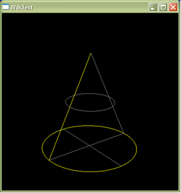
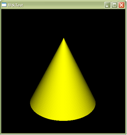
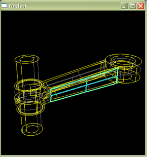
 1.8.13